Biplanar Videoradiography Dataset for Model-based Pose Estimation Development and New User Training

Lauren Welte; Andrew Dickinson; Anton Arndt; Michael J. Rainbow

doi:10.3791/63535

JoVE Journal > Engineering

Ingénierie

Biplanar Videoradiography Dataset for Model-based Pose Estimation Development and New User Training

Published: May 11, 2022

doi:

10.3791/63535

Lauren Welte¹, Andrew Dickinson¹, Anton Arndt^2,3, Michael J. Rainbow¹

¹Mechanical & Materials Engineering,Queen’s University, ²Swedish School of Sport and Health Sciences, ³Karolinska Institute

Summary

This work presents an in vivo dataset with bone poses estimated with marker-based methods. A method is included here to train operators in improving their initial estimates for model-based pose estimation and reducing inter-operator variability.

Abstract

Measuring the motion of the small foot bones is critical for understanding pathological loss of function. Biplanar videoradiography is well-suited to measure in vivo bone motion, but challenges arise when estimating the rotation and translation (pose) of each bone. The bone’s pose is typically estimated with marker- or model-based methods. Marker-based methods are highly accurate but uncommon in vivo due to their invasiveness. Model-based methods are more common but are currently less accurate as they rely on user input and lab-specific algorithms. This work presents a rare in vivo dataset of the calcaneus, talus, and tibia poses, as measured with marker-based methods during running and hopping. A method is included to train users to improve their initial guesses into model-based pose estimation software, using marker-based visual feedback. New operators were able to estimate bone poses within 2° of rotation and 1 mm of translation of the marker-based pose, similar to an expert user of the model-based software, and representing a substantial improvement over previously reported inter-operator variability. Further, this dataset can be used to validate other model-based pose estimation software. Ultimately, sharing this dataset will improve the speed and accuracy with which users can measure bone poses from biplanar videoradiography.

Introduction

Measuring the movement of the small foot bones is critical for understanding pathological loss of function. However, dynamic foot bone motion measurement is challenging due to the small size and densely packed configuration of the bones and joints¹^,². Biplanar videoradiography (BVR) technology is well-suited to measure the in vivo three-dimensional (3D) motion of the small bones of the foot and ankle during dynamic activities. BVR provides insights into arthro-kinematics by using two x-ray sources coupled to image intensifiers, which convert x-rays of dynamic motion to visible light. As the foot moves through the capture volume, high-speed cameras capture the images. The images are un-distorted and projected into the capture volume using calibrated camera positions³^,⁴. The six degrees of freedom (6 d. o. f.) bone pose (3 d.o.f. for position and 3 d.o.f. for orientation) is then estimated using either marker-based or model-based methods³.

The marker- or model-based pose estimation methods vary among laboratories and disciplines. The gold standard of dynamic BVR pose measurement is the implantation of small tantalum markers into the bone of interest⁴^,⁵. A minimum of three markers per bone is required to estimate the pose, with additional markers leading to higher accuracy⁵^,⁶. This method is less common in vivo due to its invasiveness, as it requires surgical implantation, and the markers are then embedded permanently in the bone⁷. Alternatively, model-based tracking uses volumetric information from other imaging modalities, such as computed tomography (CT) or magnetic resonance imaging, to recreate the model on the BVR images²^,³^,⁸^,⁹^,¹⁰^,¹¹^,¹²^,¹³^,¹⁴^,¹⁵. The model is then semi-manually manipulated to best match the images (rotoscoping), typically using a combination of user input as an initial estimation and cross-correlative optimization³^,⁸^,⁹^,¹⁰^,¹⁵. Model-based pose estimation is less invasive, and therefore more common, but has a greater processing time and requires user input. As the rotoscoping process is currently semi-manual, there remains a need to reliably train operators in the lab-specific software as inter-operator root mean square (RMS) errors can range from 0.83 mm to 4.96 mm, and 0.58° to 10.29° along or about a single axis¹. Further, model-matching algorithms are improving, but require validation using experimental paradigms that are as close to in vivo conditions as possible.

The accuracy of model-based pose estimations is often assessed against marker-based metrics. For example, human cadaveric feet implanted with markers have been moved through simulated locomotory positions¹³^,¹⁴^,¹⁶. The captured BVR images are then fed to the model-based rotoscoping method and compared to the marker-based metrics for accuracy (bias and precision). While the use of a static cadaver foot is a valuable approach, it has limitations in assessing true in vivo bone pose accuracy. For example, joint positions are relatively constant in a cadaver foot with the absence of muscular activity and in vivo loads. Thus, it may not represent the limits of joint motion in diverse locomotor tasks. Variations in joint posture change the occlusion in the BVR images, which is a source of measurement error when estimating small, densely packed foot bone poses¹³. Further, when using image-matching algorithms, the presence of markers in the BVR images would likely bias the results. While groups have removed the markers from the computed tomography (CT) digital imaging and communications in medicine (DICOM) images⁹^,¹⁴^,¹⁶, they are only occasionally also removed from the biplanar videoradiography images¹⁶.

This work presents an open-source BVR dataset of a participant hopping and running in vivo, who has markers implanted in his foot and ankle bones (Figure 1). Marker-based pose estimation for the in vivo bone motion of the tibia, talus, and calcaneus is provided. The markers were removed from both the x-ray and CT images to limit any bias introduced during the assessment of model-based tracking accuracy. This dataset is intended for assessing the accuracy of any model-based pose estimation software, and for improving the selection of initial pose estimates for semi-manual processes. It is most appropriate for individuals who aim to improve the speed and accuracy of the BVR image processing pipeline, and for laboratories that desire low inter-operator variability in initial pose estimation.

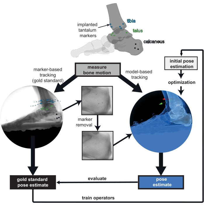
Figure 1: Overview of the provided biplanar videoradiography (BVR) dataset. Implanted markers are tracked in vivo as the gold standard for bone pose estimation. The markers were digitally removed from the BVR images and the computed tomography scans to prevent bias in the model-based tracking. Poses estimated from any model-based tracking software can be compared to the gold standard of marker-based tracking. The marker-based pose estimate can also be used to train new operators to improve their initial bone pose estimation for model-based tracking. Please click here to view a larger version of this figure.

Protocol

Experimental protocols were approved by Queen's University Health Sciences and Affiliated Teaching Hospitals Research Ethics Board. The participant gave informed consent prior to participation in the data collection.

1. Patient preparation and dataset generation

NOTE: The participant (male, 49 years, 83 kg, 1.75 m tall) had several 0.8 mm diameter tantalum markers previously implanted into the calcaneus (3 markers), talus (4 markers), and tibia (5 markers; Figure 1).

Acquire a CT scan with a metal artifact reduction algorithm (to reduce the image distortion due to metal implants) on the participant's foot in a maximally plantarflexed ankle posture with a pixel size of 0.500 mm or less, and a slice thickness of 0.625 mm or less.
NOTE: Here, the participant's right foot was scanned at a resolution of 0.441 mm x 0.441 mm x 0.625 mm. The markers' locations are not placed at specific anatomical locations within the bone⁴; instead, they are distributed throughout the bone⁵.
For methods for collecting biplanar videoradiography and processing the data in detail, see¹⁷. Briefly, ask the participant to complete the desired movement, with their start position curated such that their foot lands in the biplanar videoradiography volume. Use a calibration object and un-distortion grids to locate the cameras and un-distort the images, respectively¹⁸.
NOTE: The participant in this study completed trials of two different movements. They hopped to a metronome at 108 bpm and jogged slowly through the volume. Images were captured continuously at 250 Hz with a 1111 µs shutter speed, and the x-ray system was set to 70 kV and 100 mA.
Individually segment the markers using 3D medical image processing software. Using the content-aware fill algorithm in the raster graphics editor and the known marker locations, remove the markers from the DICOM images. Create the bone partial volumes and tessellated meshes by segmentation of the marker-less images as shown in¹⁷. Align both the partial volumes and the meshes and store them in CT space.
For each frame, tabulate the unfiltered x-y image coordinates of each marker in XMALab and export it¹⁸. Triangulate the 3D coordinates using the computer vision toolbox in MATLAB. Estimate the pose by matching the 3D marker positions in x-ray space to the sphere-fit centroids in CT space using a least-squares approach¹⁹. Use the same algorithm in the raster graphics editor to remove the markers in the x-ray images to prepare them for tracking.

2. Access the dataset and code

Download the dataset from here. There are BVR images and calibration files for each trial, as well as reference pose estimates saved in the .tra format (Figure 2). Download/clone the code package from: https://github.com/skelobslab/JOVE_BVR_FootModelAndMarkerBased.

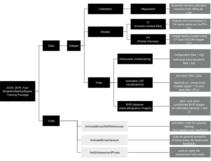
Figure 2: Data tree of the JOVE_BVR_Foot_ModelAndMarkerBased training package. Folders are shown in black boxes, code is shown in light grey boxes, and descriptions of files are contained in dark grey boxes. Please click here to view a larger version of this figure.

3. Assess the accuracy of the model-tracking algorithm

Save pose estimates as a .tra file in the trial's reference folder. Arrange the .tra file with the pose from bone space to x-ray space written in a 1-row x 16-column format, with each row corresponding to the frame and the 4 x 4 pose matrix written out as [first column, second column, third column, and fourth column].
NOTE: Bone space is synonymous with CT space in this dataset.
Verify pose estimates by opening the script verifyAssessmentPoses.m in the computing platform and then clicking Run. Load the files as described by the prompts. The script will calculate the helical axis between the model- and marker-based pose estimate and return a rotation and translation difference for each frame of tracked data.

4. New operator training

NOTE: This section describes the training with feedback for a new operator. Here, Autoscoper is the selected model-based pose estimation software, but other software could be used as a replacement.

Download the latest version of the pose estimation software from: https://simtk.org/projects/autoscoper.
To locate local BVR files, open the file in a text-editor (.JOVE_BVR_Foot_ModelAndMarkerBasedDataSOL001AT0019_jog0001AutoscoperPOINTER_T0019_jog001.cfg). The software uses a pointer file (.cfg) to locate files. Modify the directories so that they lead to the appropriate local files. Save the file and close it.
To load the BVR images and camera information, open the pose estimation software and click Load Trial. Navigate to the pointer configuration file saved in the previous step and click Open.
To track, follow the protocol in Akhbari et al¹⁷ (model-based tracking). In brief, rotate and translate the bone by clicking and dragging the axes on the bone until satisfied with the position and orientation of the calcaneus. Press the S key on the keyboard to save the current frame for the calcaneus (cal).
NOTE: Filter settings are included in JOVE_BVR_Foot_ModelAndMarkerBasedDataSOL001AT0019_jog0001Autoscoper which can be used for filtering as shown in Akhbari et al¹⁷.
To save the files, click Save Tracking. Save the file as [Trial number]_[Subject Number]_[Trial name]_[3 letter bone code].tra (e.g., T0019_SOL001A_jog0001_cal.tra) under the desired directory. Export the settings as current, matrix, column, comma, none, mm, degrees.
NOTE: The three-letter bone codes for the tibia and talus are tib and tal, respectively.
To create files for tracking accuracy, open the computing platform and run the animateBonesWithReferences.m script in the code folder. Navigate to the folders within the training package as requested by the dialog boxes.
NOTE: The animateBonesWithReferences.m code is a specialized code for training that provides the poses from marker-based data as feedback to improve the new operator's tracking.
Install visualization software from: https://github.com/DavidLaidlaw/WristVisualizer/tree/master. To visualize the tracking, open the .pos file created in step 4.6 in the visualization software; its file location will be in the computing platform’s command window.
Verify the alignment of the tracked bone (grey) with the reference bone. Green color indicates the pose is within the rotation and translation thresholds while red indicates it is outside the threshold. Continue tracking and visualizing until all frames are green. Change the thresholds (phi – rotation, trans – translation) in lines 10 and 11 of the animateBonesWithReferences.m script, if required.
NOTE: If the reference bone is red (Figure 3A), it means the pose is more than 1 mm or 2° away from the marker-based pose, as measured using the helical axis. If it is green, and visually is reasonable, that frame is tracked sufficiently well (Figure 3B).
To track the other bones in the ankle complex, repeat steps 4.4 to 4.8 for the talus and tibia. Use the visualization software to ensure that the bones are not colliding.
To complete the assessment, track and visualize the tibia, talus, and calcaneus in the trial called assessment trial.
1. Open the computing platform and run the code animateBonesGeneral.m. Navigate to the folders within the training package as requested by the dialog boxes. Verify the bone poses using the .pos file in the visualization software. This code is generalizable to other trials for 3D visualization of the bones.
  NOTE: The true, marker-based pose will no longer be available. Only the grey bones will be present.
To evaluate the pose estimates, open the script verifyAssessmentPoses.m in the computing platform and click Run. The script will calculate the helical axis between the model- and marker-based pose estimate and return a rotation and translation difference for each frame of tracked data. This will produce the same graph as in animateBoneswithReferences.m but will not produce an animation.
Verify that all data points are below the selected threshold (flat line) for both rotation and translation. Save the results out in a .csv file, if required.

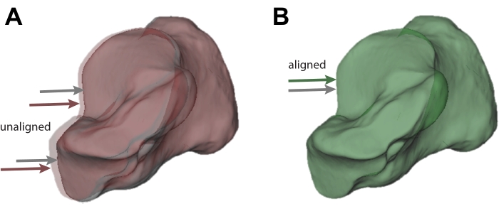
Figure 3: Visualization of acceptable and unacceptable tracking. (A) Calcaneus bone tracked using model-based tracking (grey; also indicated by the grey arrow) that does not sufficiently match the pose from the marker-based pose estimate (red; also indicated by the red arrow). (B) Calcaneus that sufficiently matches the pose from the marker-based pose estimate. The marker-tracked calcaneus is shown in green as a result (also indicated by the grey and green arrows). Please click here to view a larger version of this figure.

Representative Results

Two new operators and one expert completed the model-based training. The 41 frames of the assessment trial measured the proficiency of their model-based tracking (Figure 4). The operators' pose estimates were typically well below the set thresholds. The mean median bias (range) in rotation across bones was 0.75° (0.69° to 0.85°) for the calcaneus, 0.40° (0.37° to 0.46°) for the talus, and 0.89° (0.76° to 1.07°) for the tibia. The mean median translation bias was 0.10 mm (0.05 mm to 0.16 mm) for the calcaneus, 0.31 mm (0.22 mm to 0.41 mm) for the talus, and 0.33 mm (0.27 mm to 0.37 mm) for the tibia. These results suggest that the tutorial is effective at training the operators to within a set tolerance.

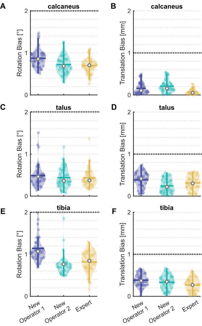
Figure 4: Rotation and translation bias for new operators and an expert. Violin plots²⁰ showing bias in (A)(C)(E) rotation and (B)(D)(F) translation between model-based and marker-based pose estimates for two new operators and one expert for the (A)(B) calcaneus, (C)(D) talus, and (E)(F) tibia. All 41 frames of the assessment trial are shown as data points, with the median (white circle), interquartile range (thick vertical line), and mean (thick horizontal line). The black line at 2° and 1 mm represent the selected thresholds. Six frames outside the threshold for New Operator 2 in (E) are not shown. Please click here to view a larger version of this figure.

One new operator had six frames above the 2° rotation threshold in their tibia tracking. The frames were identified using one of the generated graphs in verifyAssessmentPoses.m (Figure 5). These six frames are more difficult to track due to tibia occlusion by the other foot swinging through the view.

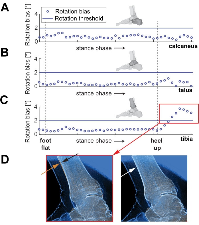
Figure 5: Rotation bias for each frame over stance phase. Example of the second new operator's rotation tracking over part of stance phase of running, for (A) the calcaneus, (B) the talus, and (C) the tibia. Note the red box in (C) shows the frames with high errors. (D) On the left, a representative image shows the approximate difference in alignment of the orange and blue lines of the anterior tibia (indicated by orange and black arrows). The right image shows an example of a well-tracked tibia (indicated by the white arrow). Please click here to view a larger version of this figure.

Supplemental File. Please click here to download this File.

Discussion

Accurate model-based pose estimation is fundamental to measuring arthro-kinematics and skeletal motion. Previous validation methods for pose estimation have been based on cadaveric specimens with implanted markers, without in vivo loading and joint ranges of motion. This in vivo dataset of running and hopping with marker-based pose estimation enables validation of model-based algorithms. Further, the dataset is organized to train new operators, such that the initial estimate required for most model-based algorithms is within a set tolerance, reducing inter-operator variability. MATLAB code is provided such that the bones can be animated and pose quality feedback is automatically generated.

The new operators were successfully trained to within a set tolerance of 2° of rotation and 1 mm of translation. These limits are much lower than reported inter-operator reliability, which can be as large as 5 mm and 10°¹. However, the selected tolerances are 2x to 4x higher than the RMS error of other intact cadaveric foot experiments (0.59 mm and 0.71°¹⁶). The tolerances include the higher-end ranges of RMS error, but still represent a substantial improvement over reported inter-operator variability. Further, in vivo conditions are more challenging to track than static foot postures due to variation in occlusion of bones, soft tissue, and artifacts of high-speed movement through the x-ray volume. The new operators successfully rotoscoped the trials within the tolerance and were close to the expert's results, except for the six frames shown in Figure 5C. Thus, the set tolerance represents an improvement over reported inter-operator variability, and the results show that this method can successfully train new operators within that tolerance.

A critical step in this protocol is the iteration between rotoscoping in the selected software and visualizing in 3D. This iteration is important for understanding how the bones are oriented in space. It allows the operator to verify if the bone poses are biologically feasible and not colliding with other bones. Continually alternating between rotoscoping and visualization improves the quality of final bone pose estimates and helps catch optimization errors.

The training set, particularly the assessment trial, includes challenging tracking scenarios to push the limits of the new operators. The position of the x-ray sources and image intensifiers in this collection caused the swinging foot to occlude the views, creating challenges for aligning the bone models. The new operator, with several frames above the rotation threshold, was affected by the contralateral foot obscuring the view. Strategies such as changing the filter settings and rotoscoping the frames immediately before and after the occlusion can help mitigate these issues. Furthermore, the orientation of the coordinate systems differs sufficiently between the DICOMs and the pose estimation software, causing an angle flip in the tibia. The operators must track every frame at this point to overcome this challenge. These scenarios are not uncommon in data collections and represent challenges that automatic model-based pose estimation should navigate in the future and are thus a valuable addition to this dataset.

There are certain limitations with this protocol. First, declaring the marker-based pose estimation as the gold standard is contentious as the accuracy difference between marker- and model-based pose estimation is not typically an order of magnitude different²^,³^,¹⁰. However, it is probable that the visual changes in BVR images that arise with in vivo collections (i.e., movement artifact, soft tissue, and bone occlusion) are more likely to induce errors in model-based pose estimation compared to marker-based methods. Further experimentation is required to confirm this hypothesis. In addition, this dataset does not capture every biplanar x-ray collection. The orientation of the cameras, such that the bones are in different relative positions, could change bone feature prominence and correspondingly affect the pose matching algorithm's cost function. Further, these features may be affected by the image filter settings¹⁵^,¹⁷. Thus, this dataset is not necessarily a generalizable assessment of BVR accuracy. Instead, it is a tool for training users to input appropriate initial pose estimates and for improving model-based pose estimation algorithms until manually rotoscoped initial guesses are no longer needed.

Divulgations

The authors have nothing to disclose.

Acknowledgements

This work was funded by the NSERC Discovery Grant (RGPIN/04688-2015) and the Ontario Early Researcher Award.

Materials

Autoscoper	Brown University		https://simtk.org/projects/autoscoper; pose estimation software
Code	Queen's University		https://github.com/skelobslab/JOVE_BVR_FootModelAndMarker Based
Content-Aware Fill algorithm, Photoshop	Adobe
Dataset	Queen's University		Download here
MATLAB	Mathworks	n/a	computing platform
Mimics	Materialise, Belgium		3D image processing software
Revolution HD	General Electric Medical Systems		CT scan device used
WristVisualizer	Brown University		https://github.com/DavidLaidlaw/WristVisualizer/tree/master; Visualization software
XMALab	Brown University		https://bitbucket.org/xromm/xmalab/src/master/

References

Maharaj, J. N., et al. The reliability of foot and ankle bone and joint kinematics measured with biplanar videoradiography and manual scientific rotoscoping. Frontiers in Bioengineering and Biotechnology. 8 (106), (2020).
Iaquinto, J. M., et al. Model-based tracking of the bones of the foot: A biplane fluoroscopy validation study. Computers in Biology and Medicine. 92, 118-127 (2018).
Miranda, D. L., et al. Static and dynamic error of a biplanar videoradiography system using marker-based and markerless tracking techniques. Journal of Biomechanical Engineering. 133 (12), 121002 (2011).
Tashman, S., Anderst, W. In-vivo measurement of dynamic joint motion using high speed biplane radiography and CT: application to canine ACL deficiency. Journal of Biomechanical Engineering. 125 (2), 238-245 (2003).
Brainerd, E. L., et al. X-ray reconstruction of moving morphology (XROMM): precision, accuracy and applications in comparative biomechanics research. Journal of Experimental Zoology Part A: Ecological Genetics and Physiology. 313 (5), 262-279 (2010).
Challis, J. H. A procedure for determining rigid body transformation parameters. Journal of Biomechanics. 28 (6), 733-737 (1995).
Lundberg, A., Goldie, I., Kalin, B. O., Selvik, G. Kinematics of the ankle/foot complex: plantarflexion and dorsiflexion. Foot & ankle. 9 (4), 194-200 (1989).
You, B. -. M., Siy, P., Anderst, W., Tashman, S. In vivo measurement of 3-D skeletal kinematics from sequences of biplane radiographs: Application to knee kinematics. IEEE Transactions on Medical Imaging. 20 (6), 514-525 (2001).
Bey, M. J., Zauel, R., Brock, S. K., Tashman, S. Validation of a new model-based tracking technique for measuring three-dimensional, in vivo glenohumeral joint kinematics. Journal of Biomechanical Engineering. 128 (4), 604-609 (2006).
Anderst, W., Zauel, R., Bishop, J., Demps, E., Tashman, S. Validation of three-dimensional model-based tibio-femoral tracking during running. Medical Engineering & Physics. 31 (1), 10-16 (2009).
Martin, D. E., et al. Model-based tracking of the hip: implications for novel analyses of hip pathology. The Journal of Arthroplasty. 26 (1), 88-97 (2011).
Massimini, D. F. Non-invasive determination of coupled motion of the scapula and humerus-An in-vitro validation. Journal of Biomechanics. 44 (3), 408-412 (2011).
Ito, K., et al. Direct assessment of 3D foot bone kinematics using biplanar X-ray fluoroscopy and an automatic model registration method. Journal of Foot and Ankle Research. 8 (1), 1-10 (2015).
Wang, B., et al. Accuracy and feasibility of high-speed dual fluoroscopy and model-based tracking to measure in vivo ankle arthrokinematics. Gait & Posture. 41 (4), 888-893 (2015).
Akhbari, B., et al. Accuracy of biplane videoradiography for quantifying dynamic wrist kinematics. Journal of Biomechanics. 92, 120-125 (2019).
Cross, J. A., et al. Biplane fluoroscopy for hindfoot motion analysis during gait: A model-based evaluation. Medical Engineering & Physics. 43, 118-123 (2017).
Akhbari, B., Morton, A. M., Moore, D. C., Crisco, J. J. Biplanar videoradiography to study the wrist and distal radioulnar joints. JoVE Journal of Visualized Experiments. (168), e62102 (2021).
Knörlein, B. J., Baier, D. B., Gatesy, S. M., Laurence-Chasen, J. D., Brainerd, E. L. Validation of XMALab software for marker-based XROMM). Journal of Experimental Biology. 219 (23), 3701-3711 (2016).
Söderkvist, I., Wedin, P. -. &. #. 1. 9. 7. ;. Determining the movements of the skeleton using well-configured markers. Journal of Biomechanics. 26 (12), 1473-1477 (1993).
Violin Plots for Matlab. Available from: https://github.com/bastibe/Violinplot-Matlab (2021)