Automated Segmentation of Cortical Grey Matter from T1-Weighted MRI Images

Eileanoir B. Johnson; Rachael I. Scahill; Sarah J. Tabrizi

doi:10.3791/58198

JoVE Journal > Neuroscience

神経科学

Automated Segmentation of Cortical Grey Matter from T1-Weighted MRI Images

Published: January 07, 2019

doi:

10.3791/58198

Eileanoir B. Johnson¹, Rachael I. Scahill¹, Sarah J. Tabrizi¹

¹Huntington’s Disease Research Centre,UCL Institute of Neurology

概要

This protocol describes the process of applying seven different automated segmentation tools to structural T1-weighted MRI scans to delineate grey matter regions that can be used for the quantification of grey matter volume.

Abstract

Within neuroimaging research, a number of recent studies have discussed the impact of between-study differences in volumetric findings that are thought to result from the use of different segmentation tools to generate brain volumes. Here, processing pipelines for seven automated tools that can be used to segment grey matter within the brain are presented. The protocol provides an initial step for researchers aiming to find the most accurate method for generating grey matter volumes from T1-weighted MRI scans. Steps to undertake detailed visual quality control are also included in the manuscript. This protocol covers a range of potential segmentation tools and encourages users to compare the performance of these tools within a subset of their data before selecting one to apply to a full cohort. Furthermore, the protocol may be further generalized to the segmentation of other brain regions.

Introduction

Neuroimaging is widely used in both clinical and research settings. There is a current move to improve the reproducibility of studies that quantify brain volume from magnetic resonance imaging (MRI) scans; thus, it is important that investigators share experiences of using available MRI tools for segmenting MRI scans into regional volumes, to improve the standardization and optimization of methods¹. This protocol provides a step-by-step guide to using seven different tools to segment the cortical grey matter (CGM; grey matter which excludes subcortical regions) from T1-weighted MRI scans. These tools were previously used in a methodological comparison of segmentation methods², which demonstrated variable performance between tools on an Huntington's disease cohort. Since performance of these tools is thought to vary among different datasets, it is important for researchers to test a number of tools before selecting only one to apply to their dataset.

Grey matter (GM) volume is regularly used as a measure of brain morphology. Volumetric measures are generally reliable and able to discriminate between healthy controls and clinical groups³. The volume of different tissue types of brain regions is most often calculated using automated software tools that identify these tissue types. Thus, to create high quality delineations (segmentations) of the GM, accurate delineation of the white matter (WM) and cerebrospinal fluid (CSF) is critical in achieving accuracy of the GM region. There are a number of automated tools that may be used for performing GM segmentation, and each requires different processing steps and results in a different output. A number of studies have applied the tools to different datasets to compare them with one other, and some have optimized specific tools¹^,⁴^,⁵^,⁶^,⁷^,⁸^,⁹^,¹⁰^,¹¹. Previous work has demonstrated that variability between volumetric tools can result in inconsistencies within the literature when studying brain volume, and these differences have been suggested as driving factors for false conclusions being drawn about neurological conditions¹.

Recently, a comparison of different segmentation tools in a cohort that included both healthy control participants and participants with Huntington's disease was performed. Huntington's disease is a genetic neurodegenerative disease with a typical onset in adulthood. Gradual atrophy of subcortical and CGM is a prominent and well-studied neuropathological feature of the disease. The results demonstrated variable performance of seven segmentation tools that were applied to the cohort, supporting previous work that demonstrated variability in findings depending on the software used to calculate brain volumes from MRI scans. This protocol provides information on the processing used in Johnson et al. (2017)² that encourages careful methodological selection of the most appropriate tools for use in neuroimaging. This manual covers the segmentation of GM volume but does not cover the segmentation of lesions, such as those seen in multiple sclerosis.

Protocol

Note: Ensure that all images are in NifTI format. Conversion to NifTI is not covered here.

1. Segmentation via SPM 8: Unified Segment

NOTE: This procedure is performed via the SPM8 GUI which operates within Matlab. The SPM8 guide provides further detail and can be found at: http://www.fil.ion.ucl.ac.uk/spm/doc/spm8_manual.pdf.

Make sure that SPM8 is installed and set in the software path.
SPM segmentation is performed using a GUI. To open SPM, open a command window and type 'spm' into the command line.
Press 'PET & VBM' to open the structural MRI toolbox.
Press 'Batch' to open the Batch Editor. This allows segmentation to be performed on multiple scans at a time.
Select 'SPM | Spatial | Segment'.
Click 'Data | Select Files'. Choose the T1-weighted scans as input.
NOTE: The files must be unzipped NifTi files, with the extension being '.nii'.
Click on 'output files | Grey Matter' and ensure that 'Native Space' is selected, do the same for White Matter. If the CSF segmentation is not required leave this as 'None'.
If the scans have already been bias-corrected, change the 'Bias Corrected' option to 'Don't Save Corrected'. For the 'Clean up any partitions' option, test the three different options and use visual quality control (QC, Section 8) to determine which works best for the data.
Leave the other settings as their defaults. Then, click on the green flag to run the segmentation.
NOTE: This takes around 5 minutes per participant, and the command line will say, 'Running Segment'. When finished, the command window will display 'Done'.
Perform visual QC on the GM (C1*.nii file) as described in Section 8.

2. Segmentation via SPM 8: New Segment

NOTE: This procedure is performed via the SPM8 GUI. The SPM8 guide provides further detail and can be found at: http://www.fil.ion.ucl.ac.uk/spm/doc/spm8_manual.pdf. Make sure that SPM8 is installed and set in the software path. Open the SPM software, typically performed by typing "spm" into a command line. This opens a graphical user interface (GUI) window with a range of options that can be selected to perform analysis.

Press 'PET & VBM'.
Press 'Batch' to open the Batch Editor.
Select 'SPM | Tools | New Segment' in the Batch window. Select the T1 image files (with extension '.nii').
Set 'Native Tissue type' to 'Native Space'. As needed, turn off the different tissue classes (such as CSF) – if not required – by setting them to 'None'. Set 'Warped Tissue' to 'None'.
NOTE: All other options can be left as the default setting.
Click the green flag to run the segmentation.
NOTE: The command line will say, 'Running New Segment'. Once it has finished running the MATLAB command line will say, 'Done New Segment'.
Perform visual QC on the GM (C1*.nii file) as described in Section 8.

3. Segmentation via SPM 12: Segment

NOTE: This procedure is performed via the SPM12 GUI. The SPM12 guide provides further detail and can be found at:http://www.fil.ion.ucl.ac.uk/spm/doc/manual.pdf.

Open the SPM software by typing 'spm' into the command window. This opens a graphical user interface (GUI) window with a range of options that can be selected to perform analysis.
Press 'PET & VBM'. Press 'Batch' to open the Batch Editor.
Click on 'SPM | Spatial | Segment'. Then, click on 'Data | Volumes'.
Set 'Native Tissue type' to 'Native Space'. Turn off the tissue classes that are not required (such as CSF) by setting them to 'None'. Set 'Warped Tissue' to 'None'.
NOTE: All other options can be left as default setting.
Click the green flag to run the segmentation.
NOTE: The command window will display: 'Running Segment'. Once the run is complete, it will display: 'Done Segment'.
Perform visual QC on the GM (C1*.nii file) as described in Section 8.

4. Segmentation via FSL FAST

NOTE: This procedure is done in the command line. The FSL guide provides further detail and can be found at: https://fsl.fmrib.ox.ac.uk/fsl/fslwiki.

Run BET brain extraction. This may need to be optimized for different datasets, but the basic command is:
bet T1_ID.nii bet_T1_ID.nii
Run FSL FAST segmentation:
fast bet_T1_ID.nii
NOTE: This will output partial volume maps and binary regions for GM, CSF, and WM.
Perform visual QC on the GM region (the file ending *_pve_1.nii.gz) as described in Section 8.

5. Segmentation via FreeSurfer

NOTE: This procedure is done in the command line. The FreeSurfer guide provides further detail and can be found at: https://surfer.nmr.mgh.harvard.edu/.

Set the directory where the data is by typing:
export SUBJECTS_DIR=/path/to/nii/files
Run the segmentation by running the commands:
recon-all -i T1_ID.nii -subjid T1_ID -autorecon1 -cw256
recon-all -subjid T1_ID -autorecon2 -autorecon3
NOTE: The commands take > 10 h per participant. The -cw256 flag is needed to crop scans with fields of view larger than 256 down to this size for processing.
Check that processing has completed correctly by looking at the script located in the 'output folder | scripts | recon-all.log'. Check that the last line says 'recon-all -s T1_ID finished without error'.
Perform visual QC on the GM region as described in Section 8.

6. Segmentation via ANTs

NOTE: This procedure is done in the command line. ANTs is a more complex software than the other tools and it should be noted that the procedure explained here could be further optimised for each cohort to improve the results. ANTs documentation can be found at: http://stnava.github.io/ANTsDoc/. There are two ways to segment the images into tissue classes as described below.

To use the first method, run the command 'antsAtropos.sh' with default settings and without including tissue priors.
NOTE: This often performs well especially when only 3 tissue classes are required: GM, WM, other.
1. Set the path to ANTs software by typing the command:
  export ANTSPATH=/path/to/ANTs/bin/
2. Run the segmentation pipeline by typing the command:
  antsAtroposN4.sh -d <image_dimension> -a <t1.nii.gz> -c <number of tissue classes> -o <output>
  1. Optional arguments for this command are:
    Brain mask: -x <mask.nii.gz>;
    Tissue priors: -p <segmentationPriors%d.nii.gz>.
3. This will create a folder with the output including partial volume maps and an extracted brain. Perform visual QC on the GM region as described in Section 8.
To generate more tissue classes (GM, subcortical GM, WM, CSF, other, etc.) or perform the segmentation on a cohort showing neural pathology, use specific tissue priors. Download tissue priors from different websites. Alternatively, use a study-specific template to make priors – this is much more complex but can be beneficial, especially in cohorts with pathological brain changes.
1. To create a study-specific template/priors, first create a study-specific template:
  antsMultivariateTemplateConstruction.sh -d <image_dimension> -o template <other options> <images.nii.gz>
  1. Optional arguments for this command are:
    -c: control for parallel computation.
    If running in serial, use a 0; -j: number of cores; -r: do rigid-body registration of inputs before creating template (default 0) — 0 == off 1 == on. This is only useful when an initial template is not available.
2. Download a brainmask and priors from the ANTs website.
  NOTE: This mask may need to be edited to make sure it is a good approximation of the template brain. The brainmask is one of the most important parts of the pipeline; if it is poor, then brain extraction/Atropos will run poorly. Some of the download options are:
  https://figshare.com/articles/ANTs_ANTsR_Brain_Templates?915436.
  The downloaded template should then be registered to the study template.
3. Calculate the registration, which will output a series of warps that can then be applied to the downloaded template to transform it to study-specific template space. To calculate the registration, use the command:
  antsRegistrationSyNQuick.sh -d 3 -f template.nii.gz -m downloaded_template.nii.gz -o downloaded_to_template -n 6
  1. The options in this command are:
    -d: dimension (i.e., 3D scans would be '3'); -f: fixed image (i.e., the space where the images need to end up); -m: moving image (i.e., the image that needs to be moved); -o: output name (no extension needed); -n: number of threads.
4. Apply the registration to the data:
  antsApplyTransforms -d 3 -i downloaded_template.nii.gz -r template.nii.gz -o downloaded_to_template.nii.gz -t downloaded_to_template1Warp.nii.gz -t downloaded_to_template0GenericAffine.mat.
  1. The options in this command are:
    -d: dimension (i.e., 3D scans would be '3'); -i: input image (i.e., the image that needs to be moved); -r: reference image (i.e., the reference image defines the spacing, origin, size, and direction of the output warped image); -o output name, this is the downloaded template in the study-specific template space (extension needed in this case); -t transform file name, the output file from the registration calculation.
5. Visually check the registration for correspondence between the study-specific template and downloaded template (to do this, open the study-specific template on top of the downloaded template).
6. If the registration has worked, apply the transformation to the downloaded priors and extracted template brain, repeating step 6.2.5.
  NOTE: Following these steps, there will be a study-specific template, a downloaded template aligned with the study-specific template, along with a downloaded brain extraction mask and tissue priors also aligned with the study-specific template.
7. Run the study specific template through antsCorticalThickness.sh; this provides GM, WM, and CSF regions that can be used for study-specific priors:
  antsCorticalThickness.sh -d 3 -a template.nii.gz -e downloaded_to_template.nii.gz -m downloaded_binarised_template_extracted_brain_in_studyspace.nii.gz -p downloaded_labelsPriors%d.nii.gz -o CT_template
  1. The options in this command are:
    -d: dimension (i.e., 3D scans would be '3'); -a: image to be segmented (in this case, the study-specific template); -e: brain template (not skull stripped; in this case, the downloaded template that has been registered to the study-specific template); -m: downloaded brain extraction mask (in this case, the extracted brain from the downloaded template that has been registered to the study-specific template); -p: priors specified using c-style formatting (e.g., -p labelsPriors%02d.nii.gz).
    NOTE: The command assumes that the first four priors are ordered as follows: 1: CSF, 2: cortical GM, 3: WM, and 4: subcortical GM (in this case, the priors from the downloaded template that has been registered to the study-specific template).
8. Running this command will result in generated priors for the template, but they need smoothing prior to use in Atropos segmentation. The smoothing command is part of ANTs software. Smooth all priors using the command:
  SmoothImage 3 CT_template_BrainSegmentationPosteriors2.nii.gz CT_template_BrainSegmentationPosteriors_smoothed.nii.gz
9. Prior to running Atropos, run brain extraction on all native space scans. The study-specific template can be used, and extracted brain generated from running antsCorticalThickness.sh on the template (step 6.2.1):
  antsBrainExtraction.sh -d 3 -a T1.nii.gz -e template.nii.gz -m template_BrainExtractionBrain.nii.gz -o T1_brain.nii.gz
  1. The options in this command are:
    -d: dimensions; -a: anatomical image; -e: brain extraction template (i.e., template created, without skull stripping); -m: study specific brainmask used for brain extraction; -o: output prefix.
10. Then run Atropos:
  antsAtroposN4.sh -d 3 -a T1.nii.gz -x T1_brain.nii.gz -c 3 -o Atropos_specific_template
  1. The options in this command are:
    -d = dimensions; -a: anatomical image; -x: brain extraction mask generated from the brain extraction; -c: number of tissue classes to segment; -o: output prefix; -p: study-specific segmentation priors <segmentationPriors%d.nii.gz>
11. Perform visual QC on the GM region as described in Section 8.

7. Segmentation via MALP-EM

To run MALP-EM, open a terminal window, change the directory into the MALP-EM install directory and type:
./malpem-proot -i T1_scan.nii -o ./ -m optional_brain_mask_final.nii.gz -f 3T -t 6 -c
Once the command has been completed, check that there is an output folder with tissue classes and regional segmentations.
Perform visual QC on the GM as described in Section 8.

8. Visual Quality Control

NOTE: Visual quality control should be performed on all segmented regions to be used in the analysis. Quality control ensures that the segmentations are of a high standard and represent reliable segmentation of the CGM. To perform quality control, each scan is opened and overlaid on the original T1 to compare the generated region to the CGM visible on the scan.

SPM, FSL, ANTs, and MALP-EM Segmentations
1. Perform visual QC using FSLeyes:
  https://users.fmrib.ox.ac.uk/~paulmc/fsleyes_userdoc/
  Note: FSLview (an older viewer) can also be used in the same way.
2. Open a terminal window and open the T1 and the GM regions overlaid on the T1. To do this, type:
  fsleyes T1.nii Region1.nii Region2.nii.
3. Once FSLeyes opens, use the opacity toggle on the top pane to adjust/reduce the opacity and allow visualisation of the T1 image underneath the GM region. Change the color of the segmentation overlay via the 'color dropdown tab' in the top pane.
4. Scroll through every slice in the brain.
  NOTE: Here this is done using the coronal view, but users should use the view that they have most experience with.
5. Check every slice for regions of under- or over-estimation of the region being inspected.
  NOTE: See the representative results section for examples of good and bad segmentations.
FreeSurfer QC
1. Peform visual QC using FreeView.
  NOTE: Refer to the documentation here:
  https://surfer.nmr.mgh.harvard.edu/fswiki/FreeviewGuide/FreeviewGeneralUsage/FreeviewQuickStart.
2. Open a terminal window. To view the volumetric GM region overlaid on the T1, change directory to the subject folder and type:
  freeview ./mri/T1.mgz ./mri/aparc+aseg.mgz:colormap=lut:opacity:.3
3. Scroll through every slice in the brain.
  NOTE: Here this is done using the coronal view, but users should use the view that they have most experience with.
4. Check every slice for regions of under- or over-estimation of the region being inspected.
  NOTE: See the representative results section for examples of the segmentations.

Representative Results

Average brain volumes for 20 control participants, along with demographic information, is shown in Table 1. This acts as a guide for expected values when using these tools. Results should be viewed in the context of the original T1.nii image. All GM regions should be inspected as per the steps described in section 8. When performing visual QC, it is important to directly compare the GM regions to the T1 scan by viewing them overlaid on the T1.

Regions should be rejected for gross errors as shown in Figure 1. Sometimes these errors result if processing was run incorrectly, or if the brain was poorly positioned within the field of view. To correct these errors, the native T1 scans can be rigidly re-aligned to standard space and segmentation can be re-attempted. The rate of failures will vary depending on quality of the data and tools used, as well as the classification of failure. In the current study, failure rates of total failures resulting in rejection were < 5% for all tools, but less significant errors were consistently seen across a number of tools. FSL FAST, SPM 8 New Segment and FreeSurfer had errors (but not failures) in > 50% of scans for this cohort. This error rate was quantified by examining the notes taken during the visual QC process, with errors included if they were seen as a reasonable departure from the expected regions, as shown in Figures 2-6. It is important to note that these tools have been validated on other datasets and result in much lower error rates ³^,⁸. While these errors could possibly be improved via manual intervention or inclusion of a mask at brain extraction, since SPM New Segment and MALP-EM resulted in a lower error rate for this dataset, these tools would be used instead. Masks can be applied before processing within ANTs and MALP-EM, and after processing for SPM (all versions) and FSL FIRST.

More minor errors are shown in Figures 2-6. By testing different segmentation tools on a dataset before application to the whole cohort, the tool that performs best on that dataset can be selected for analysis. When performing QC, a procedure should be developed for choosing to reject, edit, or accept segmentations. Common errors seen for the seven tools are described here, with examples shown in Figures 2-6. Errors in segmentation such as these can often be corrected with the addition of a mask in the processing stream or editing the regions. However, regions with extensive over- or under-estimation of the cortex may need to be rejected from analysis. Strict criteria should be developed and followed when making this decision. These steps are not covered in this protocol and will vary from dataset to dataset.

Generally, when performing visual QC, it is important to pay particular attention to temporal and occipital regions, as these are areas that show the most consistent errors. Figure 2 shows examples of good and bad temporal segmentations, and Figure 3 shows examples of good and bad occipital segmentations. Figure 4 shows another common issue that occurs in all tools, in which non-brain tissue is classified as CGM in superior slices of the brain. Figure 5 displays another issue seen in a number of segmentations where regions of the CGM are excluded from the segmentation. This often occurs in superior slices of the brain, as seen in Figure 5.

SPM8 Unified Segment commonly resulted in poor temporal delineation, with the segmented GM region spilling into non-brain tissue surrounding the temporal lobes. Spillage into the occipital lobe is common, while under-estimation of the frontal lobes also seen in a number of regions. For SPM8 New segment, poor temporal delineation and occipital spillage were also common. Using this version of SPM also results in voxels within the skull and dura being classified as GM in nearly all segmentations. SPM12 was improved compared to earlier versions of SPM, with the temporal lobe segmentations improved and less spillage in other regions. ANTs showed highly variable performance on this cohort, with the initial brain extraction determining the quality of segmentation. It is important to pay particular attention to the external boundaries, and if brain extraction is poor using ANTs, then the brain mask included in the Atropos command can be improved. Issues with over-estimation of the GM in the temporal and occipital lobes were again common. MALP-EM showed fewer issues with over-estimation of the temporal and occipital lobes; although, there was under-estimation of the cortex in a number of cases. This can be improved by inclusion of a brain mask in the pipeline. FSL FAST segmentations were highly variable, due to the variable performance of BET brain extraction on the data from this cohort. Again, issues within occipital and temporal lobes were common; however, these can be improved with optimization of brain extraction. Finally, FreeSurfer volumetric regions are often tight along the GM/CSF boundary, typically excluding some regions of GM in the outer boundary (Figure 6). As with other tools, spillage outside of the GM is prevalent within the temporal and occipital lobes. Finally, Figure 7 shows an example of a good segmentation displayed in FSLview that had no errors in segmentation. Manual editing of the regions can often be performed to improve regions, although this is not covered here.

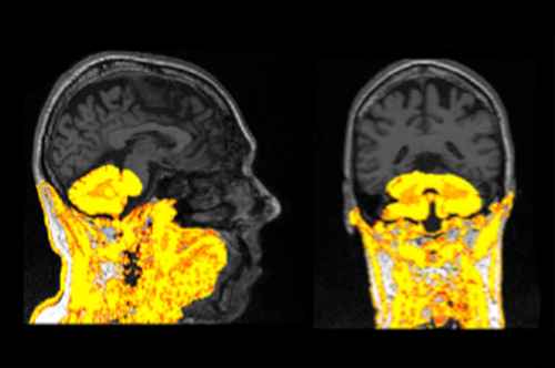
Figure 1: Example of a failed segmentation displayed on a T1 scan. This segmentation should be re-processed and excluded from analysis if it cannot be improved. Please click here to view a larger version of this figure.

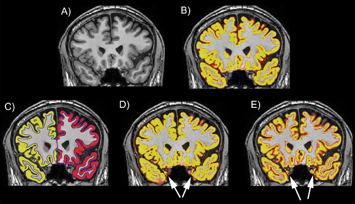
Figure 2: Examples of the performance of different tools on the temporal lobe on a T1 scan. (A) The T1 scan without a segmentation. (B) The T1 scan with an example of a good regional delineation (MALP-EM). (C) The T1 scan with an example of a good regional delineation (FreeSurfer). (D) The T1 scan with an example of a poor regional delineation, showing spillage in the left and right temporal lobes (SPM 8 New Segment). (E) The T1 scan with an example of a poor regional delineation, showing spillage in the left and right temporal lobes (FSL FAST). The scans are viewed in FSLeyes with the T1 scan as a base image and the GM region as an overlay. In this figure, the GM regions are viewed as red-yellow with an opacity of 0.4. The color gradient represents partial volume of voxels, with voxels that are more yellow having a higher PVE estimate (more likely to be GM) and those that are red having a lower PVE estimate (less likely to be GM). Please click here to view a larger version of this figure.

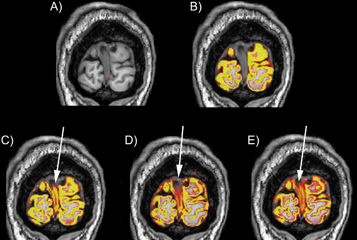
Figure 3: Examples of the performance of different tools on the occipital lobe on a T1 scan. (A) The T1 scan without a segmentation. (B) The T1 scan with an example of a good regional delineation (MALP-EM). (C) The T1 scan with an example of a poor occipital lobe delineation with spillage into the dura in the medial section of the region (SPM 8 Unified Segment). (D) The T1 scan with an example of a poor occipital lobe delineation with spillage into the dura in the medial and superior sections of the region (SPM 8 New Segment). (E) The T1 scan with an example of a poor occipital lobe delineation with spillage into the dura in the medial and superior sections of the region (FSL FAST). The scans are viewed in FSLeyes with the T1 scan as a base image, and the GM region as an overlay. In this figure, the GM regions are viewed as red-yellow with an opacity of 0.4. The color gradient represents partial volume of voxels, with voxels that are more yellow having a higher PVE estimate (more likely to be GM) and those that are red having a lower PVE estimate (less likely to be GM). Please click here to view a larger version of this figure.

Figure 4: Example of a GM region spilled into the dura, displayed in an FSLview window (in sagittal, coronal, and axial views). The blue region highlights spillage into the dura. Please click here to view a larger version of this figure.

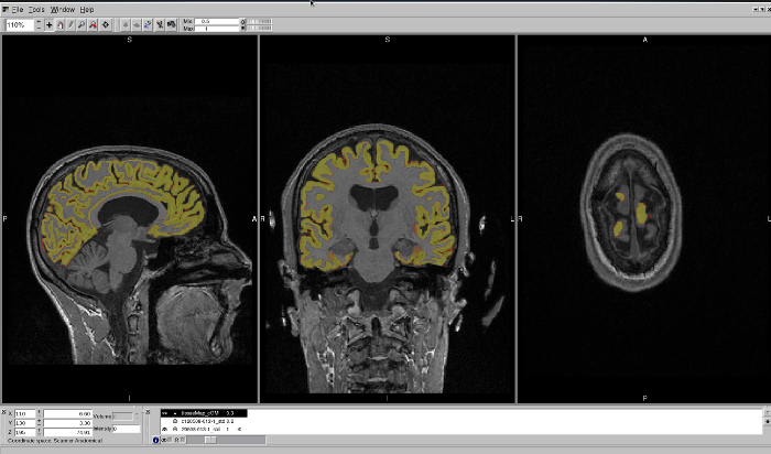
Figure 5: Example of a GM region that has excluded regions of the CGM from segmentation. This region is displayed in an FSLview window, in sagittal, coronal, and axial views. The axial view best shows the regions that have been excluded from segmentation. Please click here to view a larger version of this figure.

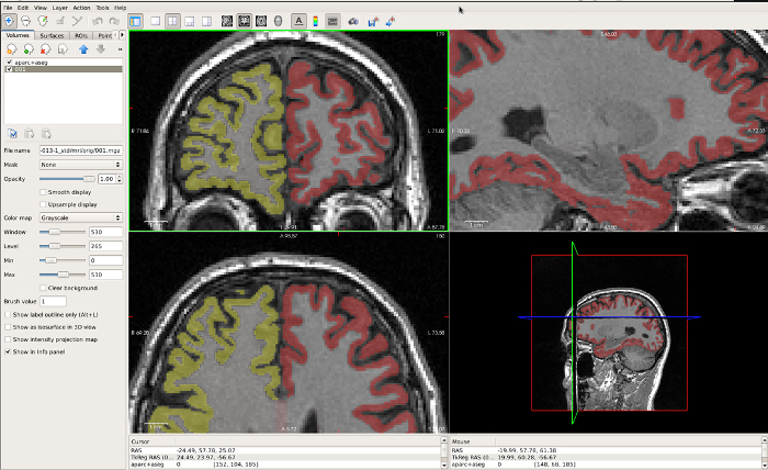
Figure 6: Example of a FreeSurfer GM region that is very tight along the GM/CSF boundary, displayed in FreeView. The coronal window in the top left best displays the under-estimation in the CGM in this region. Please click here to view a larger version of this figure.

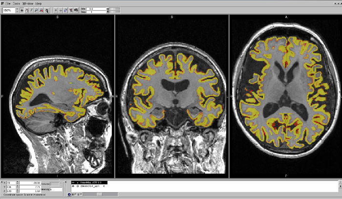
Figure 7: Example of a well-delineated MALP-EM region on a T1 brain scan. The region shows no issues with over- or under-estimation of the CGM in any region. Please click here to view a larger version of this figure.

Table 1: Demographic information and average GM volumes (mL) for 20 control participants from the TRACK-HD study, segmented using the seven tools described here.

Discussion

Recently, research has demonstrated that the use of different volumetric methods may have important implications for neuroimaging studies¹^,². By publishing protocols that help guide novice users in how to apply different neuroimaging tools, as well as how to perform QC on the results output by these tools, researchers may select the best method to apply to their dataset.

While most steps in this SOP can be adjusted to suit the data and researcher requirements, one of the most critical processes presented here are the steps describing detailed visual quality control. Visual QC should be performed on all segmentations output by these tools and is essential for the accurate measurement of CGM. The QC steps taken to ensure high-quality segmentations have been developed after the examination of thousands of CGM regions. By comparing different tools via visual examination, the most accurate method can be found for each dataset.

For each tool, there are different options that can be used to optimize segmentation on each dataset. It is often preferable to realign all scans to native space prior to segmentation, as this can reduce errors in segmentation; however, this is not essential. Furthermore, the regions output by each tool differ, with some including only cortical GM and some also including subcortical regions. Furthermore, some regions output partial volume estimates (PVE) and some output discrete tissue maps. While volume extraction is not covered here, and discussion of the difference between PVE and discrete tissue maps is beyond the scope of this standard operating procedure (SOP), PVE maps are generally accepted as a more reliable measure¹². This SOP provides information on the processing used in Johnson et al. (2017)² to segment and QC the scans; however, there may be more appropriate selections for other users depending on the quality of their images, and further processing such as the application of masks to limit regions to cortical GM may be required. All segmentations can be performed in native space.

This protocol provides example pipelines for seven different methods that can be used to segment the CGM from T1 MRI scans. These examples largely follow the default pipelines that are recommended for each software, and it is important to note that further optimization of these pipelines may be necessary for the successful segmentation of a region on different scans. Some tools, such as MALP-EM, have limited options and are likely better for users who are new to neuroimaging. Other tools, including ANTs, can undergo detailed optimization, and the protocol presented here represents one possible application of this software. Additional options, such as the use of masks to limit calculation of the volumes, are also possible for most tools.

It is important to note that not all tools can be used on every operating system. SPM and ANTs are compatible with Windows, Mac, and Linux systems, FSL is compatible with Mac and Linux systems, and MALP-EM and FreeSurfer are compatible with Linux systems (or a Linux virtual machine running on a Windows/Mac PC).

This protocol covers the steps that can be used to perform segmentation and quality control (QC) on 3D T1-weighted MRI scans to generate CGM regions. However, the protocol assumes that images are 3D T1 images in NifTI format (.nii extension). In the analysis performed by Johnson et al.², images were already bias-corrected using the N3 procedure¹³. This protocol also assumes that the software has been downloaded and installed on a linux machine as per the instructions provided by each tool. The software compared here include SPM8¹⁴, SPM12, FSL¹⁵, FreeSurfer¹⁶^,¹⁷, ANTs¹⁸, and MALP-EM¹⁹.

This SOP covers a range of segmentation techniques; however, there are other options available for segmenting structural T1 scans. These methods were selected for previous comparison by Johnson et al.² based on their frequency of use within Huntington's disease research. However, every tool performs differently in each dataset, and segmentation tools not covered here may be appropriate for other datasets and research groups.

These tools are widely used within neuroimaging research. As software updates are created for these tools, it is likely that the output of each segmentation method will undergo significant changes over time. However, emphasis should remain on the process of visual QC to ensure that high-quality segmentations are used in neuroimaging studies.

開示

The authors have nothing to disclose.

Acknowledgements

We wish to thank all those at the CHDI/High Q Foundation responsible for the TRACK-HD study; in particular, Beth Borowsky, Allan Tobin, Daniel van Kammen, Ethan Signer, and Sherry Lifer. The authors also wish to extend their gratitude to the TRACK-HD study participants and their families. This work was undertaken at UCLH/UCL, which received a proportion of funding from the Department of Health's National Institute for Health Research Biomedical Research Centres funding scheme. S.J.T. acknowledges support of the National Institute for Health Research through the Dementias and Neurodegenerative Research Network, DeNDRoN.

TRACK-HD Investigators:
C. Campbell, M. Campbell, I. Labuschagne, C. Milchman, J. Stout, Monash University, Melbourne, VIC, Australia; A. Coleman, R. Dar Santos, J. Decolongon, B. R. Leavitt, A. Sturrock, University of British Columbia, Vancouver, BC, Canada; A. Durr, C. Jauffret, D. Justo, S. Lehericy, C. Marelli, K. Nigaud, R. Valabrègue, ICM Institute, Paris, France; N. Bechtel, S. Bohlen, R. Reilmann, University of Münster, Münster, Germany; B. Landwehrmeyer, University of Ulm, Ulm, Germany; S. J. A. van den Bogaard, E. M. Dumas, J. van der Grond, E. P. 't Hart, R. A. Roos, Leiden University Medical Center, Leiden, Netherlands; N. Arran, J. Callaghan, D. Craufurd, C. Stopford, University of Manchester, Manchester, United Kingdom; D. M. Cash, IXICO, London, United Kingdom; H. Crawford, N. C. Fox, S. Gregory, G. Owen, N. Z. Hobbs, N. Lahiri, I. Malone, J. Read, M. J. Say, D. Whitehead, E. Wild, University College London, London, United Kingdom; C. Frost, R. Jones, London School of Hygiene and Tropical Medicine, London, United Kingdom; E. Axelson, H. J. Johnson, D. Langbehn, University of Iowa, IA, United States; and S. Queller, C. Campbell, Indiana University, IN, United States.

参考文献

Katuwal, G. J., et al. Inter-Method Discrepancies in Brain Volume Estimation May Drive Inconsistent Findings in Autism. Frontiers in Neuroscience. 10, 439 (2016).
Johnson, E. B., et al. Recommendations for the Use of Automated Gray Matter Segmentation Tools: Evidence from Huntington’s disease. Frontiers in Neurology. 8, 519 (2017).
Schwarz, C. G., et al. A large-scale comparison of cortical thickness and volume methods for measuring Alzheimer’s disease severity. NeuroImage: Clinical. 11, 802-812 (2016).
Clarkson, M. J., et al. A comparison of voxel and surface based cortical thickness estimation methods. NeuroImage. 57 (3), 856-865 (2011).
Eggert, L. D., Sommer, J., Jansen, A., Kircher, T., Konrad, C. Accuracy and reliability of automated gray matter segmentation pathways on real and simulated structural magnetic resonance images of the human brain. Public Library of Science One. 7 (9), 45081 (2012).
Fellhauer, I., et al. Comparison of automated brain segmentation using a brain phantom and patients with early Alzheimer’s dementia or mild cognitive impairment. Psychiatry Research. 233 (3), 299-305 (2015).
Gronenschild, E. H. B. M., et al. The effects of FreeSurfer version, workstation type, and Macintosh operating system version on anatomical volume and cortical thickness measurements. Public Library of Science One. 7 (6), 38234 (2012).
Iscan, Z., et al. Test-retest reliability of freesurfer measurements within and between sites: Effects of visual approval process. Human Brain Mapping. 36 (9), 3472-3485 (2015).
Kazemi, K., Noorizadeh, N. Quantitative Comparison of SPM, FSL, and Brainsuite for Brain MR Image Segmentation. Journal of Biomedical Physics & Engineering. 4 (1), 13-26 (2014).
Klauschen, F., Goldman, A., Barra, V., Meyer-Lindenberg, A., Lundervold, A. Evaluation of automated brain MR image segmentation and volumetry methods. Human Brain Mapping. 30 (4), 1310-1327 (2009).
McCarthy, C. S., Ramprashad, A., Thompson, C., Botti, J. A., Coman, I. L., Kates, W. R. A comparison of FreeSurfer-generated data with and without manual intervention. Frontiers in Neuroscience. 9, (2015).
Tohka, J. Partial volume effect modeling for segmentation and tissue classification of brain magnetic resonance images: A review. World Journal of Radiology. 6 (11), 855-864 (2014).
Sled, J. G., Zijdenbos, A. P., Evans, A. C. A nonparametric method for automatic correction of intensity nonuniformity in MRI data. IEEE Transactions on Medical Imaging. 17, 87-97 (1998).
Ashburner, J., Friston, K. J. Unified segmentation. NeuroImage. 26 (3), 839-851 (2005).
Jenkinson, M., Beckmann, C., Behrens, T. E., Woolrich, M. W., Smith, S. M. FSL. NeuroImage. 62, 782-790 (2012).
Dale, A. M., Fischl, B., Sereno, M. I. Cortical surface-based analysis. I. Segmentation and surface reconstruction. NeuroImage. 9, 179-194 (1999).
Fischl, B., Sereno, M. I., Dale, A. M. Cortical surface-based analysis. II: Inflation, flattening, and a surface-based coordinate system. NeuroImage. 9, 195-207 (1999).
Avants, B. B., Tustison, N. J., Wu, J., Cook, P. A., Gee, J. C. An open source multivariate framework for n-tissue segmentation with evaluation on public data. Neuroinformatics. 9 (4), 381-400 (2011).
Ledig, C., et al. Robust whole-brain segmentation: application to traumatic brain injury. Medical Image Analysis. 21 (1), 40-58 (2015).

Play Video

PDF

DOI

記事を引用

Johnson, E. B., Scahill, R. I., Tabrizi, S. J. Automated Segmentation of Cortical Grey Matter from T1-Weighted MRI Images. J. Vis. Exp. (143), e58198, doi:10.3791/58198 (2019).

Automated Segmentation of Cortical Grey Matter from T1-Weighted MRI Images