Statistical Modelling of Cortical Connectivity Using Non-invasive Electroencephalograms
Summary
Standard EEG analysis techniques offer limited insight into nervous system function. Deriving statistical models of cortical connectivity offers far greater ability to investigate underlying network dynamics. Improved functional assessment opens new possibilities for diagnosis, prognostication, and outcome prediction in nervous system diseases.
Abstract
Non-invasive electrophysiological recordings are useful for the evaluation of nervous system function. These techniques are inexpensive, fast, replicable, and less resource-intensive than imaging. Further, the functional data produced have excellent temporal resolution, which is not achievable with structural imaging.
Current applications of electroencephalograms (EEG) are limited by data processing methods. Standard analysis techniques using raw time series data at individual channels are very limited methods of interrogating nervous system activity. More detailed information about cortical function can be achieved by examining relationships between channels and deriving statistical models of how areas are interacting, allowing visualization of connectivity between networks.
This manuscript describes a method for deriving statistical models of cortical network activity by recording EEG in a standard manner, then examining the interelectrode coherence measures to assess relationships between the recorded areas. Higher order interactions can be further examined by assessing the covariance between the coherence pairs, producing high-dimensional "maps" of network interactions. These data constructs can be examined to assess cortical network function and its relationship to pathology in ways not achievable with traditional techniques.
This approach offers greater sensitivity to network level interactions than is achievable with raw time series analysis. It is, however, limited by the complexity of drawing specific mechanistic conclusions about the underlying neural populations and the high volumes of data generated, requiring more advanced statistical techniques for evaluation, including dimensionality reduction and classifier-based approaches.
Introduction
This method aims to produce statistical maps of cortical networks based on non-invasive electrode recordings using a clinically viable setup, to allow for investigation of nervous system pathology, the impact of novel treatments, and the development of novel electrophysiological biomarkers.
EEG offers great potential for the investigation of nervous system function and disease1,2. This technology is inexpensive, readily available in research and clinical settings, and generally well tolerated. The simple, non-invasive nature of recordings make clinical use straightforward, and the existing framework of clinical EEG departments allows for easy access to the technology for clinicians.
From a technical perspective, EEG offers excellent time domain resolution3. This is of great importance when investigating nervous system function due to the rapid timescales of nervous system interactions and network dynamics. While imaging methods such as functional MRI offer greater spatial resolution and easily interpretable images, they are far more limited in their ability to interrogate nervous system function on the fine time scales offered by electrophysiological recordings4,5,6.
There is a growing need for the ability to interrogate nervous system function to inform diagnosis, treatment, and prognostication of nervous system diseases. The role of cortical network dynamics in nervous system pathology is increasingly recognized7. Many pathologies of the nervous system produce no macroscopic structural lesions visible with traditional imaging, but the abnormalities produced at the network level may be apparent with appropriate functional analysis methods.
Unfortunately, current EEG analysis methods are greatly limited in this regard. Traditional methods involve the analysis of simple time series data from individual electrodes. These signals represent the summation of field potentials in large cortical areas3,8. Analysis of data from individual channels in isolation using either visual inspection or simple statistical methods limits the usefulness of these recordings to detecting gross electrophysiological abnormalities in discrete, individual locations. With the increasing recognition of the importance of network-level effects to nervous system function and pathology, these simple analysis methods are clearly deficient in that they will fail to detect subtle relationships between signals, representing abnormalities in how cortical areas are interacting with one another at the network level.
A method of deriving statistical maps of cortical network connectivity from low-dimensional electrode recordings is demonstrated. This method allows investigation of the dynamics of interactions between varying brain regions in a way that is not possible with traditional analysis techniques, as well as visualization of these network interactions. This opens the possibility for non-invasive investigation of network level effects at high time domain resolutions in ways not previously possible. This method is based on the derivation of measures of interelectrode coherence9,10. These measures allow the investigation of how two recorded regions are interacting by evaluating the statistical relationships between the recordings of these areas11. By assessing how each recorded area interacts with every other recorded area, a statistical map of electrophysiological networks within the recorded areas can be made. This allows for the discovery of functional relationships that are not apparent on evaluation of individual channel data in isolation.
The focus of this manuscript is on the use of coherence on neural time series. Currently, there are a number of techniques for investigating the relationships between time series data that can be applied to channels in a pairwise fashion to derive models of cortical connectivity. Some methods, such as the related partial directed coherence12,13, aim to infer the direction of influence of the pair of signals investigated in order to better characterize the structure of the underlying networks, while other methods, such as Granger causality14,15, attempt to infer functional relationships through the ability of one signal to predict the data in another. Methods such as these can be applied in similar ways to generate high-dimensional models of cortical networks. However, the advantages of coherence as a means of investigating relationships between neural signals lies in its lack of assumptions. It is possible to investigate statistical relationships between recordings at two sites without making statements about the functional basis of these relationships and to build up a model of cortical connectivity based purely on statistical relationships with minimal assumptions about the cortical networks generating these signals.
Due to the purely mathematical nature of these measures, the relationship between the coherence measures of electrode recordings at the scalp and the underlying neural activity is complex16,17. While these methods allow the derivation of statistical constructs describing relationships between the electrode recordings for comparison, making direct causal inferences about the activity of the specific underlying neural populations is not straightforward3,8,16,17. These approaches allow for comparison of the network-level activity between groups to identify potentially useful biomarkers but are limited in terms of drawing specific conclusions regarding the relationship of these markers to specific neural mechanisms. This is due to the large number of confounding factors influencing the recorded activity3, as well as issues with estimating the specific cortical source of electrical signals recorded at the level of the scalp8. Rather, these approaches can produce statistical models of activity that can be interrogated and compared between groups to determine that differences exist at the network level18 and can be leveraged to produce novel biomarkers based on these constructs. However, these methods alone have a limited capacity to relate the differences seen to specific mechanisms and neural activities due to the complexity of the underlying system.
The use of network measures such as coherence is well established in systems neuroscience16,17. The full potential of these approaches for modelling and investigating cortical function has been limited by a lack of exploitation of these high-dimensional data structures. This work demonstrates that it is possible to apply these measures to EEG channels in a pairwise fashion in order to map data onto a high-dimensional feature space based purely on the statistical relationships between the electrical activity in cortical regions. It also demonstrates that, using modern statistical techniques, it is possible to use the generated models of cortical function to investigate these models without losing the information gained in the modelling process.
This method is potentially valuable in expanding the scope of applications of existing EEG technologies, improving the ability to derive useful functional measures without requiring adaptations to existing recording equipment18,19. By improving the ability to model cortical function and interrogate these models, the questions that can be investigated using EEG data are expanded. This further opens the possibility of greater integration of functional and structural evaluations for investigation of neurological disease20,21. This approach, using technology that is already widely available clinically, would allow investigation of cortical pathologies with both high temporal and spatial resolution.
Protocol
The following experimental protocol is in accordance with all local, national, and international ethics guidelines for human research. The data used to test the protocol have been acquired with authorization of the Ethical Committee of region Tuscany-protocol 2018SMIA112 SI-RE.
NOTE: The scripts used for implementing the analyses described are available at https://github.com/conorkeogh/NetworkAnalysis.
1. Raw Data Collection
- Prepare subject conditions.
- To ensure consistency across recordings, conduct all EEG recordings in a dedicated recording environment. Remove all equipment or stimuli that is not directly relevant to the task to be performed during recording from the environment to avoid distraction.
NOTE: If resting state recordings are to be performed, remove all sources of distraction from the room and expose subjects to the recording environment prior to the recording session to remove novelty from the environment. - Provide the subject with clear instructions regarding the task to be performed. Once the equipment has been set up, leave the subject alone in the recording environment to get used to the environment prior to beginning recording to minimize movement and distraction.
- If the subject has intellectual disabilities, allow him/her the necessary time to accustom to the environment to limit any stress. Sometimes this may require multiple visits and an extended stay in the recording room.
- To ensure consistency across recordings, conduct all EEG recordings in a dedicated recording environment. Remove all equipment or stimuli that is not directly relevant to the task to be performed during recording from the environment to avoid distraction.
- Mount the electrodes.
- Attach the electrode cap to the patient's head, taking care to ensure correct alignment. Inject conductive gel into each of the electrode ports, beginning at the scalp and slowly withdrawing to the cap surface to establish electrical contact with the scale and improve the signal-to-noise ratio.
- Attach electrodes to the electrode cap using a predetermined electrode montage based on the 10−20 system. Attach appropriate ground electrodes (e.g., to the mastoid processes).
- Set up the EEG.
- Connect all electrodes to an electrophysiological recording system. Link the recording system with an appropriate digital recording environment.
- Examine all the recording channels to ensure the offset is within an appropriate range and to avoid excessive channel noise. If a channel has an excessive offset or noise, additional conductive gel can be added in order to improve the electrical connection, taking care to avoid causing bridging between electrode sites.
- Instruct the subject that recording has started and to avoid all unnecessary movements. Conduct a short test recording to verify appropriate recording quality.
- Prepare the behavioral task for recording.
- Clarify all the task-related instructions with the subject. Reiterate the importance of avoiding all unnecessary movements.
- Explain that recording will begin on a clearly agreed signal (e.g., a knock on the recording environment door). Leave the subject in the recording environment. Start recording. Give the agreed signal to the subject.
- Following the completion of the task or period of resting state, stop recording, visually examine the data to ensure quality, and save the data.
2. Data Preprocessing
NOTE: The data preparation and feature extraction pipeline is illustrated in Figure 1.
- Prepare the software.
- Load the EEG data to be analyzed into a data analysis environment. Load any additional script libraries necessary, such as EEGLab22.
- Convert all recordings to the same data format if necessary, with all channels in their corresponding locations.
- Discard the beginning and end of each recording (e.g., 5 min) to reduce the contamination of movement artifacts. Split the data into epochs based on task or, if it is a resting state recording, predetermined duration (e.g., 10 min). See NetworkAnalysis_Demonstration.m (section Feature Extraction) and Supplementary Figure 1 for a demonstration of implementation.
NOTE: Selection of the epoch length can have important effects on the measures of coherence. Epochs of a sufficient length should be used to ensure that true relationships between the signals emerge in the computations to avoid unnoticed artifacts or transient, spurious synchronizations having an excessive weighting. However, in this work there was no statistically significant difference in the overall network structure when ten-minute epochs were compared to an average of ten one-minute epochs following thorough artifact rejection.
- Discard the beginning and end of each recording (e.g., 5 min) to reduce the contamination of movement artifacts. Split the data into epochs based on task or, if it is a resting state recording, predetermined duration (e.g., 10 min). See NetworkAnalysis_Demonstration.m (section Feature Extraction) and Supplementary Figure 1 for a demonstration of implementation.
- Perform artifact rejection by visually inspecting the epoch data and rejecting visually unsuitable data.
NOTE: As the modelling technique described relies on the relationships between signals, it is essential to ensure thorough rejection of artifacts. These can corrupt the channel data, leading to artificial increases (if the artifact is represented on multiple channels) or decreases (if the artifact is represented only on some channels) of measures of coherence.- Identify bad channels in the recordings.
- High pass filter data at 0.5 Hz to remove the baseline drift due to the floating ground of the acquisition system.
- Select all channels meeting the appropriate statistical criteria (e.g., those with a standard deviation greater than three times or less than one third of the average channel standard deviation).
NOTE: Removing the channels with data that are unlikely to have originated from neural sources avoids spurious relationships being introduced into the network models. - Examine these channels to determine whether they are suitable.
- Reject the epochs with unsuitable channels if possible. Alternatively, exclude the bad channels and interpolate the data at these channels (e.g., using EEGLab's spline interpolation algorithm).
NOTE: Interpolation across a large number of channels or with only a small number of recording channels may generate unsuitable data for analysis. Further, this introduces no new information into the dataset and can result in artificially high measures of coherence between interpolated signals and the signals from which they are derived.
- Perform the independent component analysis on the remaining epochs (e.g., using EEGLab's ICA function). Visually inspect the derived components and reject visually unsuitable data.
- Apply the appropriate statistical thresholds to identify the potential artifacts not immediately evident on visual inspection (e.g., based on extreme values or abnormal spectra). Examine these and determine whether rejection is appropriate.
- Repeat the independent component analysis and artifact identification on the surviving epochs.
- Identify the data epochs to be saved for further analysis. Discard all the rejected data epochs. Identify all the epochs to be taken forward for further analysis.
NOTE: Where only one epoch per subject is required, select the first suitable epoch for further analysis.
- Identify bad channels in the recordings.
- To prepare the data, correct the baseline of the recordings by subtracting the mean of all channels from the recordings to avoid the impact of baseline wandering during prolonged recordings. Re-reference all the channels to an appropriate reference (e.g., the ground electrode or the average of all channels). See NetworkAnalysis_Demonstration.m, NetworkAnalysis_Preprocess.m, and Supplementary Figure 2 for examples of implementation.
NOTE: Reference selection can have important effects on the network measures. As the reference data are "subtracted out" of all analyzed channels, any neural data that are represented on the reference channel will be subtracted out and thus not contribute to the model generation. It is common practice to use reference signals recorded over bony prominences without immediately underlying neural structures, such as the mastoid process. However, these can be corrupted by neural data due to volume conduction effects through the scalp and therefore distort network measures differentially based on location relative to the reference. As a result, for resting state data it is best to use an average of all scalp channels as reference. This means that all data are not referenced relative to a specific spatial location, distorting measures, because all channels contribute to the reference. This can have effects such as dampening the apparent overall activity and can distort measures by subtracting out signals that are very strongly represented on some channels and thus contribute heavily to the average. This is a greater issue for activity- and event-related signals, but is typically not the case with resting state data.- Digitally filter all the channels to isolate frequencies of interest (e.g., 1 Hz-50 Hz). See NetworkAnalysis_Demonstration.m, NetworkAnalysis_Preprocess.m, and Supplementary Figure 3 for examples of implementation.
NOTE: Ensure the use of appropriate frequency limits and filter parameters for the intended analysis to avoid the distortion of frequencies at the extremes of the examined range and aliasing effects. Zero phase-shift 4th-order Butterworth filters perform appropriately. Appropriate filtering ensures that the activity of interest is isolated for modelling. Even with a broad range (e.g., 1 Hz-50 Hz), this ensures that high frequency artifacts and low frequency baseline wandering are not interpreted as coherent between channels, distorting measures.
- Digitally filter all the channels to isolate frequencies of interest (e.g., 1 Hz-50 Hz). See NetworkAnalysis_Demonstration.m, NetworkAnalysis_Preprocess.m, and Supplementary Figure 3 for examples of implementation.
3. Feature Extraction
- Assess spectral power.
- Calculate overall power spectra by performing a Fourier transform of each channel being analyzed across the whole frequency range to be assessed (e.g., 1 Hz-50 Hz).
- Assess the activity in individual frequency bands: isolate the theta band at 4 Hz-8 Hz. Isolate the alpha band at 8 Hz-12 Hz. Isolate the beta band at 12 Hz-30 Hz. Isolate the delta band at 0.5 Hz-4Hz. Isolate the gamma band at >30 Hz (e.g., 30-50 Hz). See NetworkAnalysis_Demonstration.m, NetworkAnalysis_FeatureExtraction.m, and Supplementary Figure 4 for examples of the implementation of spectra derivation and isolation of frequency bands.
NOTE: EEG data are traditionally divided into frequency "bands" for investigation. These are primarily named based on the order in which they were discovered, and the specific bandwidths vary somewhat. The functional significance of oscillations at specific frequencies remains an area of active investigation. It is thought that oscillations within specific bands may be related to specific neural activities, such as the emergence of a high-amplitude alpha wave in the occipital region with the eyes closed, although the exact relationship between neural functions and oscillatory activity in EEG recordings remains unclear. - Evaluate overall power across the whole scalp by calculating the mean of individual channel spectra. Normalize the power in individual bands with respect to the overall power to give a measure of relative power and allow more accurate comparisons between conditions.
- Perform network mapping.
- Evaluate the interactions between the first electrode pair by deriving a measure of interelectrode coherence:

See NetworkAnalysis_Demonstration.m, NetworkAnalysis_FeatureExtraction.m, and Supplementary Figure 5 for examples of implementation.- Calculate the cross-spectrum of the two channels:

- Compute the Fourier transform of each signal, X and Y

- Calculate the cross-spectrum:

Where: t is the sampling interval, T is the length of recording, X is the Fourier transform of x, and Y* is the complex conjugate of Y. - Ignore the negative frequencies and correct measures. The second half of the computer frequency axis can be disregarded in the case of real-valued signals, and the power measures multiplied by two to correct for this.
NOTE: This is equivalent to the Fourier transform of the cross-correlation of x and y.
- Compute the Fourier transform of each signal, X and Y
- Normalize the cross-spectrum by the power spectra of both channels:
 .
.
- Compute the Fourier transform of each signal:

- Calculate the power spectrum:

Where: t is the sampling interval, T is the length of recording, X is the Fourier transform of x, and X* is the complex conjugate of X. - Ignore the negative frequencies and correct measures: the second half of the computer frequency axis can be disregarded in the case of real-valued signals, and the power measures multiplied by two to correct for this.
- Use the calculated power spectra to normalize the cross-spectrum and derive a measure of coherence:

NOTE: This generates C, a measure of the coherence between signals x and y at the frequencies . This is a measure of the relationship between these signals at the frequencies examined, measured on a scale from 0 to 1. Where there is a constant phase relationship between the two signals examined at all timepoints, the coherence will have a value of 1, indicating a strong relationship between signals at those frequencies, implying that activity in one signal is functionally related to activity in the other (i.e., that there is communication between the two). Where there is no phase relationship between the two signals, the coherence will have a value of 0, indicating that the signals are not related.
- Compute the Fourier transform of each signal:
- Calculate the cross-spectrum of the two channels:
- Repeat this procedure for each unique pair of electrodes to develop a measure of phase stability between the signals at each electrode pair, building up a model of functional connectivity across all electrodes.
NOTE: For a montage of n electrodes, this will produce coherence measures. This represents mapping the measured time series data onto a high-dimensional plane based on the relationships between recorded signals, allowing the nature of these interactions to be investigated.
- Evaluate the interactions between the first electrode pair by deriving a measure of interelectrode coherence:
4. Data Visualization
- Perform spectral power analysis.
- Examine the power matrices.
- Map the measurements of the spectral power to be visualized onto a two-dimensional data structure where each column is an electrode location, each row is a frequency band, and each cell is the spectral power at that location, within that band.
- Identify the maximum and minimum power levels across all conditions to be compared. Set these at the maximum and minimum for all conditions. Map the spectral power values between the identified maximum and minimum to colors. Export a color map visualizing the spectral power at each frequency band at each electrode location (Figure 2).
- Perform topographic mapping.
- Create a data structure containing the labels of each of the 10-20 system electrode locations used, in order corresponding to that of the data structure to be mapped. Using EEGLab's topoplot() function, the spectral power data, the identified maximum and minimum, and the channel list, generate a plot mapping the distribution of spectral power across the scalp.
- Examine the power matrices.
- Assess coherence.
- Examine the coherence matrices.
- Map the measurements of the interelectrode coherence to be visualized onto a two-dimensional data structure where each column is an electrode location, each row is an electrode location, and each cell is the coherence between the corresponding electrode pair.
- Map the coherence values between 0 and 1 to colors. Export a color map visualizing the interelectrode coherence between each electrode pair within the frequency limits used (Figure 3). Repeat this procedure for each frequency band to be investigated. See Supplementary Figure 6 and produce_plots.r for examples of implementation. See Figure 3 for example output.
- Perform network visualization.
- To visualize higher-order interactions between cortical areas and map out network dynamics, calculate how each electrode pair's coherence measure covaries with those of every other unique electrode pair across the overall spectrum and within specific bands.
- Map these covariance measures to colors. Export a color map visualizing the network dynamics within and across-frequency bands. See produce_plots.r for examples of implementation. See Figure 4 for example output.
- Examine the coherence matrices.
5. Analyzing Network Models
NOTE: The application of modern statistical methods to the models derived allows for taking advantage of the relationships modelled in the high-dimensional network feature space to investigate cortical function. A number of approaches that offer advantages over traditional comparisons of the individual measures or averages of the coherence measures can be taken. Some of the potential approaches these network models facilitate are outlined below. These are discussed only superficially as indicative of the potential applications of network modelling, because a thorough discussion of each technique is beyond the scope of the present work.
- Perform dimensionality reduction.
NOTE: Comparisons at the individual variable level fail to take advantage of the relationships represented by the models created, while performing comparisons on all of the measures in the dimensional constructs created is problematic due to the huge number of comparisons required and the failure to integrate the high-level information contained in the statistical models. Mapping the high-dimensional data onto a lower-dimensional space while maintaining the information generated by the model generation process allows for the performance of meaningful comparisons while taking full advantage of the models' data-rich structure.
- Derive measures for comparison between the groups that represent the overall network dynamics within the statistical models generated using the principal component analysis. See NetworkAnalysis_Demonstration.m and Supplementary Figure 7 for an example of implementation.
- As above, construct a covariance matrix for the pairwise coherence measures. This will generate a
 dimensional covariance construct where
  . This model is therefore extremely high-dimensional and allows visualization of high-level network relationships as outlined above.
 - Decompose the covariance matrix into eigenvectors and corresponding eigenvalues. This allows identification of the axes within the model feature space that contain the greatest variance, without being bounded by the existing measures.
- Rank the eigenvectors by corresponding eigenvalue to identify those accounting for the greatest proportion of variance within the model.
- As above, construct a covariance matrix for the pairwise coherence measures. This will generate a
- Compare the first principal components derived from the network models. See NetworkAnalysis_Demonstration.m and Supplementary Figure 7 for an example of implementation.
NOTE: The first principal component accounts for the greatest degree of variance within the model. Therefore, comparison of this measure allows for comparison of the overall network dynamics throughout the model as a whole between groups with a single statistical test, allowing for simultaneous analysis of the complex relationships being modelled and avoiding the issues associated with many comparisons.
- Derive measures for comparison between the groups that represent the overall network dynamics within the statistical models generated using the principal component analysis. See NetworkAnalysis_Demonstration.m and Supplementary Figure 7 for an example of implementation.
- Perform a region of interest analysis. The models derived represent network connectivity across the whole cortex, across all frequency bands. If there is interest in specific anatomical areas or in functions within specific bands, these regions of the model can be isolated and analyzed separately.
- Choose an anatomical region of interest.
NOTE: Restricting analysis to specific anatomical areas allows for evaluation of the network activity within or between specific cortical areas in order to identify the relationships that may not be apparent on analysis of the model as a whole.- Identify the coherence data within the model relating to the anatomical areas of interest.
- Derive a covariance matrix and perform principal component analysis as described above to compute measures of overall network architecture within the regions of interest.
- Compare the measures of network dynamics within the anatomical regions of interest between the groups as outlined above.
- Choose a functional region of interest.
NOTE: Restricting analysis to specific frequency bands allows for assessment of the network activity within specific oscillatory frequencies (Figure 4).- As with anatomical analyses, isolate the coherence data within the frequency bands of interest. See NetworkAnalysis_Demonstration.m and Supplementary Figure 8 for examples of implementation, using interactions within the overall spectrum only as an example.
- Perform principal component analysis to derive measures of overall network activity within the bands of interest.
- Compare the measures between groups to evaluate the network differences at specific oscillatory frequencies.
- Choose an anatomical region of interest.
- Use machine learning.
NOTE: Modern statistical learning approaches can be applied to the models generated in order to further interrogate the high-level relationships represented within them.- Use supervised learning.
NOTE: Using data with predefined classes, the models of cortical networks can be used to derive classifiers that can be used to identify signatures within the complex relationships represented by the models to classify new data, opening the possibility for investigating novel diagnostic and prognostic biomarkers, etc. Furthermore, which features within the models drive these classifications in order to gain insights into the underlying mechanisms can be investigated.- Derive the classifiers. Using pre-labelled data, a classifier can be derived to predict the class of a set of data based on the network models.
- Divide the data into a set of subject data for training and a set for testing the classifier.
- Train a classification algorithm such as a support vector machine or a random forest on the labelled training data.
- Assess the performance of the model-trained classifier on the test data.
NOTE: These approaches allow use of the statistical models as inputs to derive novel biomarkers.
- Perform sequential elimination.
NOTE: Using the model to train a classifier, data can be removed iteratively and the training process can be repeated to identify which components of the model are driving its predictive ability, allowing for investigation of the underlying mechanisms.- Train a classifier on the model as described above.
- Remove the model feature with the lowest variability between groups.
- Repeat the training process and assess performance.
- Repeat the iterative feature removal until the features that contribute most to the performance are identified. These are the model components responsible for the ability to differentiate between classes.
- Derive the classifiers. Using pre-labelled data, a classifier can be derived to predict the class of a set of data based on the network models.
- Perform unsupervised learning.
NOTE: Using the models alone, insight can be gained into the groups being investigated. By modelling the data as high-dimensional constructs based on the relationships between recordings, relationships between groups that were not seen at the level of individual recordings may become apparent. Unsupervised techniques such as clustering algorithms allow for the investigation of relationships within the models without being restricted by the predefined classes.- Using a distance metric such as Euclidean distance, compute the measures of distance between subjects within the space defined by the network model. See NetworkAnalysis_Demonstration.m and Supplementary Figure 9 for an example of implementation.
- Using a clustering algorithm such as k-nearest neighbors, identify the groups within the data based on the model parameters (Figure 5).
- Repeat this procedure using a sequential elimination procedure as described above to investigate how individual features contribute to the groupings within the model.
NOTE: This allows use of the derived models to identify the groups within the data that were not apparent otherwise. This may allow for the derivation of disease subtypes, pathological groupings, etc., that are only evident at the network level.
- Use supervised learning.
Representative Results
Measurements of the spectral power will produce n measures for each frequency band measured, where n is the number of channels recorded. These measures will be in decibels for the overall power. Measures of power within individual frequency bands should be expressed as relative power (i.e., the proportion of overall power represented by power within that band) to allow accurate comparisons between groups and conditions.
An example of visualization of spectral power across multiple bands and across recorded channels is shown in Figure 2. Spectral power can be visualized interpolated across the scalp, allowing limited estimation of the "source" of activity.
Interelectrode coherence measures produce a measure for each unique electrode pair (i.e.,  , where n is the number of channels recorded). Each of these measures is between 0 and 1, where 0 represents no coherence between recordings and 1 represents full coherence between recordings. This is a measure of the extent to which the activity in one area changes depending on the activity in another area, allowing for differences in the direction of interaction and time lag. Higher values of coherence suggest interactions between the areas, from which it is apparent that the recorded areas are communicating with each other. By measuring the interactions between every unique electrode pair, a statistical map of how the recorded channels are interacting can be built up. This allows investigation of how areas are communicating, rather than focusing on individual areas in isolation, as in traditional methods. An example of visualization of coherence measures for an 8-electrode montage is shown in Figure 3.
These coherence measures rapidly produce large volumes of data, making analysis of each measure with individual statistical tests an untenable strategy. Further, investigating individual interactions is not necessarily interesting or meaningful when considering interactions across whole cortical networks. Dimensionality reduction techniques such as principal component analysis allows for the assessment of measures from these statistical constructs to facilitate the comparisons of overall network dynamics using traditional statistical methods. Classifier-based methods, using machine learning techniques, offer an additional promising avenue for integrating these high-dimensional data constructs to classify data and predict outcomes.
Visualization of higher-order network dynamics allows recognition of the kinds of interactions being compared by a principal component analysis, or a classifier-based technique. This can be achieved using color mapping of covariance measures of the interelectrode coherence measures of electrode pairs. This evaluates how the coherence measures at one electrode pair relate to changes in coherence at another pair, suggesting broader network interactions and integration of activity across the cortex. This allows visualization of how areas are interacting in a way that is not possible with traditional measures. An example of the kind of high-dimensional network map that can be created using this technique is shown in Figure 4. This demonstrates the differences evident on network mapping between two subjects with different clinical phenotypes of a neuropsychiatric disorder affecting cortical function, where there were no statistically significant differences using standard analysis methods.
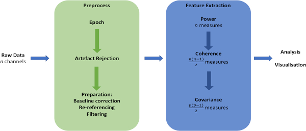
Figure 1: Schematic of data analysis pipeline. Overview of major steps in preparation of raw data and extraction of measures of interest. Please click here to view a larger version of this figure.
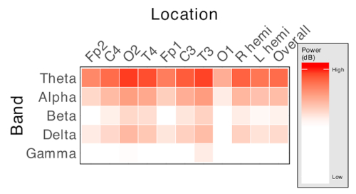
Figure 2: Representative matrix of spectral power measures. Each column represents an electrode location, and each row represents a frequency band of interest. Cell color intensity represents the value of relative power of the corresponding frequency at the corresponding electrode location. Produces n x f measures, where n is the number of recording electrodes used and f is the number of frequency bands of interest. Please click here to view a larger version of this figure.
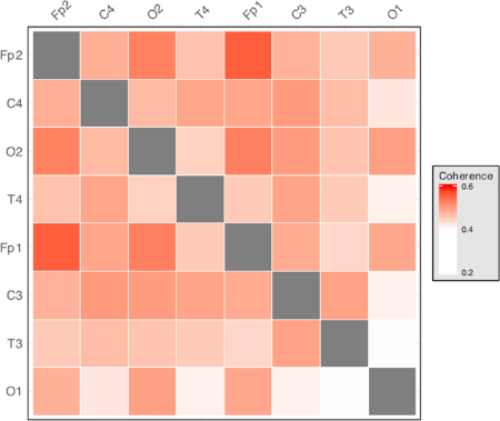
Figure 3: Representative matrix of interelectrode coherence measures. Each row and each column represents an electrode location. Cell color intensity represents the value of interelectrode coherence between the corresponding electrode pair. Produces measures for each frequency band of interest, where n is the number of recording electrodes used. Please click here to view a larger version of this figure.
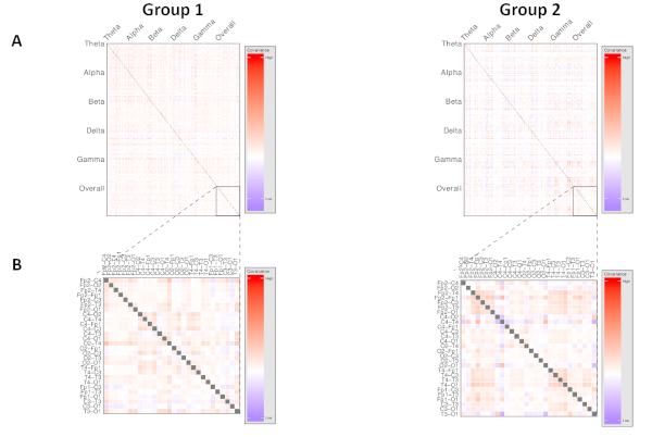
Figure 4: Representative visualization of higher-order network dynamics, comparing two phenotypes of neuropsychiatric disorder. Each row and each column represents a unique electrode pair. Cell color intensity represents the value of covariance between the corresponding electrode pairs. Produces measures for each frequency band of interest, where p is the number of unique electrode pairs used. (A) Demonstrates both within- and across-frequency interactions within cortical networks, while (B) visualizes a region of interest analysis focused on network dynamics within the overall power spectrum only. Please click here to view a larger version of this figure.
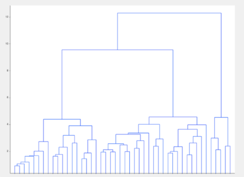
Figure 5: Representative visualization of unsupervised clustering algorithm. In a group of apparently well-matched patients with a neuropsychiatric disorder, clustering based on model data alone identified groups within the population that were not evident on standard analyses. Please click here to view a larger version of this figure.

Supplementary Figure 1: Screenshot demonstrates epoching of EEG data. Please click here to view a larger version of this figure.
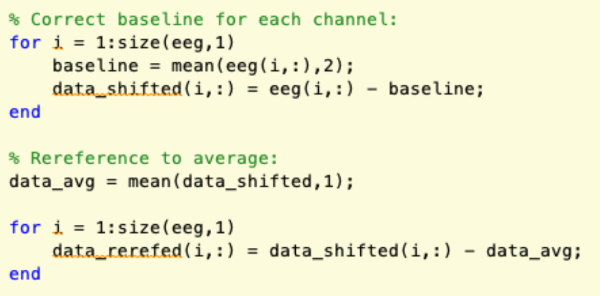
Supplementary Figure 2: Screenshot demonstrates the essential preprocessing steps. Please click here to view a larger version of this figure.
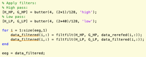
Supplementary Figure 3: Screenshot demonstrates filtering for frequencies of interest. Please click here to view a larger version of this figure.
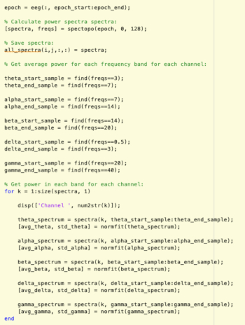
Supplementary Figure 4: Calculating channel spectra and isolating data within individual bands. Please click here to view a larger version of this figure.

Supplementary Figure 5: Calculating coherence measures for each electrode pair. Please click here to view a larger version of this figure.
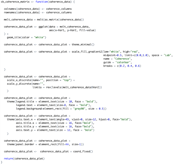
Supplementary Figure 6: Mapping derived measures to color maps and visualization. Figure 3 and Figure 4 demonstrate sample outputs. Please click here to view a larger version of this figure.
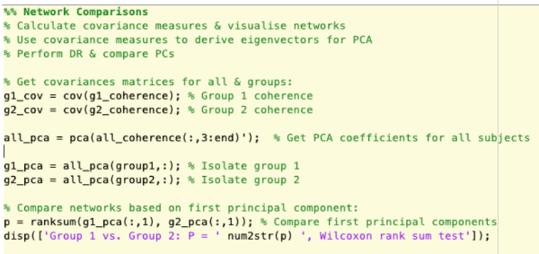
Supplementary Figure 7: Construction of covariance matrices, performing principal component analysis and comparing groups based on principal components. Please click here to view a larger version of this figure.
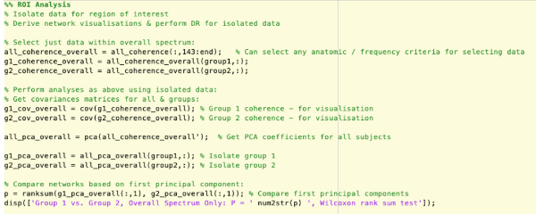
Supplementary Figure 8: Analysis of specific regions of interest by isolating subsets of data. Please click here to view a larger version of this figure.

Supplementary Figure 9: Derivation of a distance metric and use of a clustering algorithm to identify groups using unsupervised learning techniques. Please click here to view a larger version of this figure.
Discussion
The described method allows the derivation of statistical maps of cortical network dynamics from non-invasive EEG data. This allows the investigation of phenomena not readily apparent on examination of simple time series data through assessment of how the recorded regions are interacting with each other, rather than evaluating what is happening in each individual location in isolation. This can reveal important insights into disease pathology18.
The essential aspect of this method is ensuring data quality. Rigorous data evaluation, artifact rejection, and preprocessing are required to ensure data are of a sufficiently high quality to produce meaningful results. Provided the data used is of an appropriate quality, the feature extraction component can be easily modified to model network interactions in specific regions of interest only, or within arbitrary frequency limits, as well as modelling complex interactions across specific regions and frequency bands.
This approach is limited by the high-dimensionality of the produced results, which can rapidly produce huge amounts of data if many channels are used. This can limit interpretability of the raw results and result in long computation times. The use of dimensionality reduction techniques, such as principal component analysis23, is therefore necessary to allow meaningful statistical comparisons to be made between groups without needing to perform huge numbers of statistical tests. Further, the use of the produced high-dimensional network maps to aid decision making may require the use of machine learning classifiers to allow integration of the large quantities of data, which are not easily interpretable manually and cannot be easily reduced to a single measure24.
This approach offers a far greater capacity to investigate changes in network dynamics than raw EEG time series, while also offering significant advantages over imaging techniques such as functional MRI, including ease of accessibility, cost, and greater time resolution. Future applications of this method to subtyping of neurological disease, prediction of treatment response, and disease prognostication offer the possibility of greatly expanding the clinical usefulness of current clinical EEG technologies through improved data analysis methods.
Disclosures
The authors have nothing to disclose.
Acknowledgements
The publication of this manuscript has been partially supported by the SFI FutureNeruro-Funded Investigator grant to DT.
Materials
| Electrode cap | ElectroCap International | Or any suitable cap | |
| Conductive gel | SignaGel | Or any suitable gel | |
| Pin-type electrodes | BioSemi | Or any suitable electrode | |
| BioSemi Active Two recording system | BioSemi | ||
| ActiView recording environment | BioSemi | ||
| MATLAB software | Mathworks |
References
- Rosenow, F., Klein, K. M., Hamer, H. M. Non-invasive EEG evaluation in epilepsy diagnosis. Expert Review of Neurotherapeutics. 15 (4), 425-444 (2015).
- Sharmila, A. Epilepsy detection from EEG signals: a review. Journal of Medical Engineering & Technology. 42 (5), 368-380 (2018).
- Nunez, P., Srinivasan, R. . Electric Fields of the Brain: The Neurophysics of EEG. , (2006).
- Glover, G. H. Overview of functional magnetic resonance imaging. Neurosurgery Clinics of North America. 22 (2), 133-vii (2011).
- Lin, E., Alessio, A. What are the basic concepts of temporal, contrast, and spatial resolution in cardiac CT?. Journal of Cardiovascular Computed Tomography. 3 (6), 403-408 (2009).
- Kim, S., Richter, W., Uǧurbil, K. Limitations of temporal resolution in functional MRI. Magnetic Resonance in Medicine. 37, 631-636 (1997).
- Fox, M. D. Mapping Symptoms to Brain Networks with the Human Connectome. New England Journal of Medicine. 379, 2237-2245 (2018).
- Makeig, S., Bell, A., Jung, T. P., Sejnowski, T. Independent component analysis of electroencephalographic data. Advances in neural information processing systems. 8, 145-151 (1996).
- Bowyer, S. M. Coherence a measure of the brain networks: past and present. Neuropsychiatric Electrophysiology. , (2016).
- Srinivasan, R., Winter, W. R., Ding, J., Nunez, P. L. EEG and MEG coherence: measures of functional connectivity at distinct spatial scales of neocortical dynamics. Journal of Neuroscience Methods. 166 (1), 41-52 (2007).
- Bullmore, E., Sporns, O. Complex brain networks: graph theoretical analysis of structural and functional systems. Nature Reviews Neuroscience. 10, 186-198 (2009).
- Baccalá, L., Sameshima, K. Partial directed coherence: a new concept in neural structure determination. Biological Cybernetics. 84, 463-474 (2001).
- Sameshima, K., Baccalá, L. Using partial directed coherence to describe neuronal ensemble interactions. Journal of Neuroscience Methods. 94, 93-103 (1999).
- Seth, A., Barrett, A. B., Barnett, L. Granger causality analysis in neuroscience and neuroimaging. Journal of Neuroscience. 35, 3293-3297 (2015).
- Hesse, W., Möller, E., Arnold, M., Schack, B. The use of time-variant EEG Granger causality for inspecting directed interdependencies of neural assemblies. Journal of Neuroscience Methods. 124, 27-44 (2003).
- Nunez, P. L., et al. EEG coherency. I: Statistics, reference electrode, volume conduction, Laplacians, cortical imaging, and interpretation at multiple scales. Electroencephalography and Clinical Neurophysiology. 103, 499-515 (1997).
- Nunez, P. L., et al. EEG coherency II: experimental comparisons of multiple measures. Clinical Neurophysiology. 110, 469-486 (1999).
- Keogh, C., et al. Clinical and genetic Rett syndrome variants are defined by stable electrophysiological profiles. BMC Pediatrics. 18 (1), 333 (2018).
- Peters, J. M., et al. Brain functional networks in syndromic and non-syndromic autism: a graph theoretical study of EEG connectivity. BMC Medicine. 11, 54 (2013).
- Jie, B., Wee, C., Shen, D., Zhang, D. Hyper-connectivity of functional networks for brain disease diagnosis. Medical Image Analysis. 32, 84-100 (2016).
- Zhang, H., et al. Topographical Information-Based High-Order Functional Connectivity and Its Application in Abnormality Detection for Mild Cognitive Impairment. Journal of Alzheimer’s Disease. 54, 1095-1112 (2016).
- Delorme, A., Scott, M. EEGLAB: an open source toolbox for analysis of single-trial EEG dynamics including independent component analysis. Journal of Neuroscience Methods. 134, 1 (2004).
- Calabrese, B. . Encyclopedia of Bioinformatics and Computational Biology. , (2019).
- Colic, S., et al. Support Vector Machines Using EEG Features of Cross-Frequency Coupling Can Predict Treatment Outcome in Mecp2-Deficient Mice. Conference Proceedings of the IEEE Engineering in Medicine and Biology Society. , 5606-5609 (2015).

