A Virtual Machine Platform for Non-Computer Professionals for Using Deep Learning to Classify Biological Sequences of Metagenomic Data
Summary
This tutorial describes a simple method to construct a deep learning algorithm for performing 2-class sequence classification of metagenomic data.
Abstract
A variety of biological sequence classification tasks, such as species classification, gene function classification and viral host classification, are expected processes in many metagenomic data analyses. Since metagenomic data contain a large number of novel species and genes, high-performing classification algorithms are needed in many studies. Biologists often encounter challenges in finding suitable sequence classification and annotation tools for a specific task and are often not able to construct a corresponding algorithm on their own because of a lack of the necessary mathematical and computational knowledge. Deep learning techniques have recently become a popular topic and show strong advantages in many classification tasks. To date, many highly packaged deep learning packages, which make it possible for biologists to construct deep learning frameworks according to their own needs without in-depth knowledge of the algorithm details, have been developed. In this tutorial, we provide a guideline for constructing an easy-to-use deep learning framework for sequence classification without the need for sufficient mathematical knowledge or programming skills. All the code is optimized in a virtual machine so that users can directly run the code using their own data.
Introduction
The metagenomic sequencing technique bypasses the strain isolation process and directly sequences the total DNA in an environmental sample. Thus, metagenomic data contain DNA from different organisms, and most biological sequences are from novel organisms that are not present in the current database. According to different research purposes, biologists need to classify these sequences from different perspectives, such as taxonomic classification1, virus-bacteria classification2,3,4, chromosome-plasmid classification3,5,6,7, and gene function annotation (such as antibiotic resistance gene classification8 and virulence factor classification9). Because metagenomic data contain a large number of novel species and genes, ab initio algorithms, which do not rely on known databases for sequence classification (including DNA classification and protein classification), are an important approach in metagenomic data analysis. However, the design of such algorithms requires professional mathematics knowledge and programming skills; therefore, many biologists and algorithm design beginners have difficulty constructing a classification algorithm to suit their own needs.
With the development of artificial intelligence, deep learning algorithms have been widely used in the field of bioinformatics to complete tasks such as sequence classification in metagenomic analysis. To help beginners understand deep learning algorithms, we describe the algorithm in an easy-to-understand fashion below.
An overview of a deep learning technique is shown in Figure 1. The core technology of a deep learning algorithm is an artificial neural network, which is inspired by the structure of the human brain. From a mathematical point of view, an artificial neural network may be regarded as a complex function. Each object (such as a DNA sequence, a photo or a video) is first digitized. The digitized object is then imported to the function. The task of the artificial neural network is to give a correct response according to the input data. For example, if an artificial neural network is constructed to perform a 2-class classification task, the network should output a probability score that is between 0-1 for each object. The neural network should give the positive object a higher score (such as a score higher than 0.5) while giving the negative object a lower score. To obtain this goal, an artificial neural network is constructed with the training and testing processes. During these processes, data from the known database are downloaded and then divided into a training set and test set. Each object is digitized in a proper way and given a label ("1" for positive objects and "0" for negative objects). In the training process, the digitized data in the training set are inputted into the neural network. The artificial neural network constructs a loss function that represents the dissimilarity between the output score of the input object and the corresponding label of the object. For example, if the label of the input object is "1" while the output score is "0.1", the loss function will be high; and if the label of the input object is "0" while the output score is "0.1", the loss function will be low. The artificial neural network employs a specific iterative algorithm that adjusts the parameters of the neural network to minimize the loss function. The training process finishes when the loss function cannot be obviously further decreased. Finally, the data in the test set are used to test the fixed neural network, and the ability of the neural network to calculate the correct labels for the novel objects is evaluated. More principles of deep learning algorithms can be found in the review in LeCun et al.10.
Although the mathematical principles of deep learning algorithms may be complex, many highly packaged deep learning packages have recently been developed, and programmers can directly construct a simple artificial neural network with a few lines of code.
To assist biologists and algorithm design beginners in getting started in using deep learning more quickly, this tutorial provides a guideline for constructing an easy-to-use deep learning framework for sequence classification. This framework uses the "one-hot" encoding form as the mathematical model to digitize the biological sequences and uses a convolution neural network to perform the classification task (see the Supplementary Material). The only thing that the users need to do before using this guideline is to prepare four sequence files in "fasta" format. The first file contains all sequences of the positive class for the training process (referred to "p_train.fasta"); the second file contains all sequences of the negative class for the training process (referred to "n_train.fasta"); the third file contains all sequences of the positive class for the testing process (referred to "p_test.fasta"); and the last file contains all sequences of the negative class for the testing process (referred to "n_test.fasta"). The overview of the flowchart of this tutorial is provided in Figure 2, and more details will be mentioned below.
Protocol
1. The installation of the virtual machine
- Download the virtual machine file from (https://github.com/zhenchengfang/DL-VM).
- Download the VirtualBox software from https://www.virtualbox.org.
- Decompress the ".7z" file using related software, such as "7-Zip", "WinRAR" or "WinZip".
- Install the VirtualBox software by clicking the Next button in each step.
- Open the VirtualBox software and click the Nuevo button to create a virtual machine.
- Step 6: Enter the specified virtual machine name in the "Name" frame, select Linux as the operating system in the "Type" frame, select Ubuntu in the "Version" frame and click the Next button.
- Allocate the memory size of the virtual machine. We recommend that users pull the button to the right-most part of the green bar to assign as much memory as possible to the virtual machine, and then click the Next button.
- Choose the Use an existing virtual hard disk file selection, select the file "VM_Bioinfo.vdi" downloaded from Step 1.1 and then click the Create button.
- Click the Star button to open the virtual machine.
NOTE: Figure 3 shows the screenshot of the desktop of the virtual machine.
2. Create shared folders for files exchanging between the physical host and the virtual machine
- In the physical host, create a shared folder named "shared_host", and on the desktop of the virtual machine, create a shared folder named "shared_VM".
- In the Menu Bar of the virtual machine, click Devices, Shared Folder, Shared Folders Settings successively.
- Click the button in the upper right corner.
- Select the shared folder in the physical host created in Step 2.1 and select the Auto-mount option. Click the OK button.
- Restart the virtual machine.
- Click the right click on the desktop of the virtual machine and open the terminal.
- Copy the follow command to the terminal:
sudo mount -t vboxsf shared_host ./Desktop/shared_VM- When prompted for a password, enter "1" and hit the "Enter" key, as shown in Figure 4.
3. Prepare the files for the training set and test set
- Copy all four sequence files in "fasta" format for the training and testing process to the "shared_host" folder of the physical host. In this way, all the files will also occur in the "shared_VM" folder of the virtual machine. Then, copy the files in the "shared_VM" folder to the "DeepLearning" folder of the virtual machine.
4. Digitize the biological sequences using "one-hot" encoding form
- Go to the "DeepLearning" folder, click the right click and open the terminal. Type the following command:
./onehot_encoding p_train.fasta n_train.fasta p_test.fasta n_test.fasta aa
(for amino acid sequences)
or
./onehot_encoding p_train.fasta n_train.fasta p_test.fasta n_test.fasta nt
(for nucleic acid sequences)
NOTE: A screenshot of this process is provided in Figure 5.
5. Train and test the artificial neural network
- In the terminal, type the following command as shown in Figure 6:
python train.py
NOTE: The training process will begin.
Representative Results
In our previous work, we developed a series of sequence classification tools for metagenomic data using an approach similar to this tutorial3,11,12. As an example, we deposited the sequence files of the subset of training set and test set from our previous work3,11 in the virtual machine.
Fang & Zhou11 aimed to identify the complete and partial prokaryote virus virion proteins from virome data. The file "p_train.fasta" contains the virus virion protein fragments for the training set; the file "n_train.fasta" contains the virus nonvirion protein fragments for the training set; the file "p_test.fasta" contains the virus virion protein fragments for the test set; and the file "n_test.fasta" contains the virus nonvirion protein fragments for the test set. The user can directly execute the following two commands to construct the neural network:
./onehot_encoding p_train.fasta n_train.fasta p_test.fasta n_test.fasta aa
and
python train.py
The performance is shown in Figure 7.
Fang et al.3 aimed to identify phage DNA fragments from bacterial chromosome DNA fragments in metagenomic data. The file "phage_train.fasta" contains the phage DNA fragments for the training set; the file "chromosome_train.fasta" contains the chromosome DNA fragments for the training set; the file "phage_test.fasta" contains the phage DNA fragments for the test set; and the file "chromosome_test.fasta" contains the chromosome DNA fragments for the test set. The user can directly execute the following two commands to construct the neural network:
./onehot_encoding phage_train.fasta chromosome_train.fasta phage_test.fasta chromosome_test.fasta nt
and
python train.py
The performance is shown in Figure 8.
It is worth noting that because the algorithm contains some processes that have randomness, the above results may be slightly different if users rerun the script.
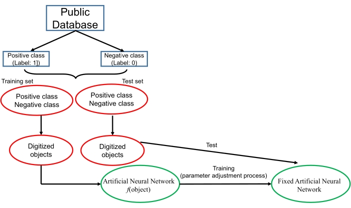
Figure 1. Overview of the deep learning technique. Please click here to view a larger version of this figure.
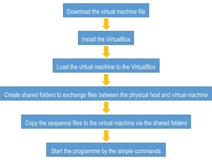
Figure 2. The overview of the flowchart of this tutorial. Please click here to view a larger version of this figure.

Figure 3. The screenshot of the desktop of the virtual machine. Please click here to view a larger version of this figure.
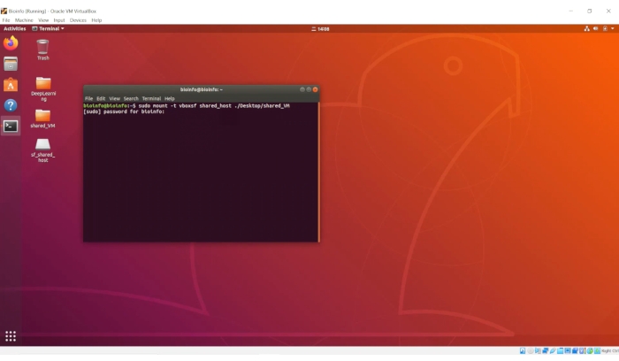
Figure 4. The screenshot of the activation of the shared folders. Please click here to view a larger version of this figure.
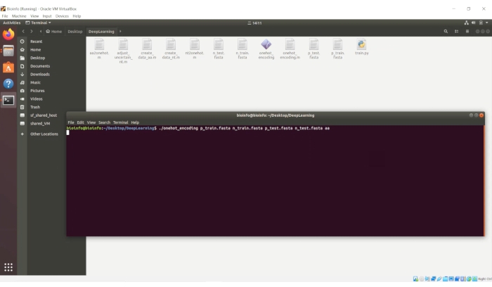
Figure 5. The screenshot of the process of sequence digitization. Please click here to view a larger version of this figure.
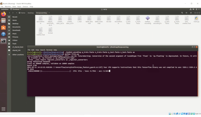
Figure 6. Train and test the artificial neural network. Please click here to view a larger version of this figure.
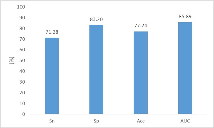
Figure 7. The performance of prokaryote virus virion protein fragments identification. The evaluation criteria are Sn=TP/(TP+FN), Sp=TN/(TN+FP), Acc=(TP+TN)/(TP+TN+FN+FP) and AUC. Please click here to view a larger version of this figure.
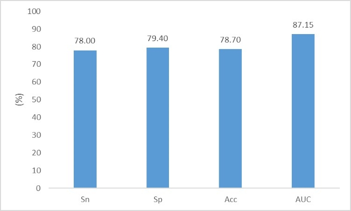
Figure 8. The performance of phage DNA fragments identification. The evaluation criteria are Sn=TP/(TP+FN), Sp=TN/(TN+FP), Acc=(TP+TN)/(TP+TN+FN+FP) and AUC. Please click here to view a larger version of this figure.
Supplementary Material: Please click here to download this file.
Discussion
This tutorial provides an overview for biologists and algorithm design beginners on how to construct an easy-to-use deep learning framework for biological sequence classification in metagenomic data. This tutorial aims to provide intuitive understanding of deep learning and address the challenge that beginners often have difficulty installing the deep learning package and writing the code for the algorithm. For some simple classification tasks, users can use the framework to perform the classification tasks.
Considering that many biologists are not familiar with the command line of the Linux operating system, we preinstalled all the dependent software in a virtual machine. In this way, the user can directly run the code in the virtual machine following the protocol mentioned above. Additionally, if users are familiar with the Linux operating system and Python programming, they can also run this protocol directly on the server or local PC. In this way, the user should preinstall the following dependent software:
Python 2.7.12 (https://www.python.org/)
Python packages:
numpy 1.13.1 (http://www.numpy.org/)
h5py 2.6.0 (http://www.h5py.org/)
TensorFlow 1.4.1 (https://www.tensorflow.org/)
Keras 2.0.8 (https://keras.io/)
MATLAB Component Runtime (MCR) R2018a (https://www.mathworks.com/products/compiler/matlab-runtime.html)
The manual of our previous work3 has a brief description of the installation. Note that the version number of each package corresponds to the version that we used in the code. The advantage of running the code in the server or local PC without the virtual machine is that the code can speed up with a GPU in this way, which can save much time in the training process. In this way, the user should install the GPU version of TensorFlow (see the manual of previous work3).
Some of the critical steps within the protocol are described as follows. In step 4.1, the file names of "p_train.fasta", "n_train.fasta", "p_test.fasta" and "n_test.fasta" should be replaced by the used file names. The order of these four files in this command cannot be changed. If the files contain amino acid sequences, the last parameter should be "aa"; if the files contain nucleic acid sequences, the last parameter should be "nt". This command uses the "one-hot" encoding form to digitize the biological sequences. An introduction of the "one-hot" encoding form is provided in the Supplementary Material. In step 5.1, because the virtual machine cannot be sped up with the GPU, this process may take a few hours or several days, depending on the data size. The progress bars for each iteration epoch are shown in the terminal. We set the number of epochs to 50, and thus, a total of 50 progress bars will be displayed when the training process is finished. When the test process is finished, the accuracy for the test set will be displayed in the terminal. In the "DeepLearning" folder of the virtual machine, a file named "predict.csv" will be created. This file contains all the prediction scores for the test data. The order of these scores corresponds to the sequence order in "p_test.fasta" and "n_test.fasta" (the first half of these scores corresponds to "p_test.fasta", while the second half of these scores corresponds to "n_test.fatsa"). If users want to make predictions for the sequences whose true classes are unknown, they can also deposit these unknown sequences either in the "p_test.fasta" or "n_test.fasta" file. In this way, the scores of these unknown sequences will also be displayed in the "predict.csv" file, but the "accuracy" display in the terminal does not make sense. This script employs a convolutional neural network to perform the classification. The structure of the neural network and the code for the neural network are shown in the Supplementary Material.
One of the characteristics of deep learning is that many parameter settings require some experience, which can be a major challenge for beginners. To avoid beginner apprehension caused by a large number of formulas, we do not focus on the mathematical principles of deep learning, and in the virtual machine, we do not provide a special parameter setting interface. Although this may be a good choice for beginners, inappropriate parameter selection may also lead to a decline in precision. To allow beginners to better experience how to modify the parameters, in the script "train.py", we add some comments to the related code, and users can modify the related parameters, such as the number of convolution kernels, to see how these parameters affect the performance.
Additionally, many deep learning programs should be run under a GPU. However, configuring the GPU also requires some computer skill that may be difficult for non-computer professionals; therefore, we choose to optimize the code in a virtual machine.
When solving other sequence classification tasks based on this guideline, users need only replace the four sequence files with their own data. For example, if users need to distinguish plasmid-derived and chromosome-derived sequences in metagenomic data, they can directly download plasmid genomes (https://ftp.ncbi.nlm.nih.gov/refseq/release/plasmid/) and bacterial chromosome genomes (https://ftp.ncbi.nlm.nih.gov/refseq/release/bacteria/) from the RefSeq database and separate the genomes into a training set and test set. It is worth noting that DNA sequences in metagenomic data are often fragmented rather than complete genomes. In such cases, users can use the MetaSim13 tool to extract the DNA fragment from the complete genome. MetaSim is a user-friendly tool with a GUI interface, and users can finish most operations using the mouse without typing any command on the keyboard. To simplify the operation for beginners, our tutorial is designed for a two-class classification task. However, we need to perform multiclassification in many tasks. In such cases, beginners can try to separate the multiclassification task into several two-class classification tasks. For example, to identify the phage host, Zhang et al. constructed 9 two-class classifiers to identify whether a given phage sequence can infect a certain host.
The homepage of this tutorial is deposited on the GitHub site https://github.com/zhenchengfang/DL-VM. Any update of the tutorial will be described on the website. Users can also raise their questions about this tutorial on the website.
Divulgaciones
The authors have nothing to disclose.
Acknowledgements
This investigation was financially supported by the National Natural Science Foundation of China (81925026, 82002201, 81800746, 82102508).
Materials
| PC or server | NA | NA | Suggested memory: >6GB |
| VirtualBox software | NA | NA | Link: https://www.virtualbox.org |
Referencias
- Liang, Q., Bible, P. W., Liu, Y., Zou, B., Wei, L. DeepMicrobes: taxonomic classification for metagenomics with deep learning. NAR Genomics and Bioinformatics. 2 (1), (2020).
- Ren, J., et al. VirFinder: a novel k -mer based tool for identifying viral sequences from assembled metagenomic data. Microbiome. 5 (1), 69 (2017).
- Fang, Z., et al. PPR-Meta: a tool for identifying phages and plasmids from metagenomic fragments using deep learning. GigaScience. 8 (6), (2019).
- Ren, J., et al. Identifying viruses from metagenomic data using deep learning. Quantitative Biology. 8 (1), 64-77 (2020).
- Zhou, F., Xu, Y. cBar: a computer program to distinguish plasmid-derived from chromosome-derived sequence fragments in metagenomics data. Bioinformatics. 26 (16), 2051-2052 (2010).
- Krawczyk, P. S., Lipinski, L., Dziembowski, A. PlasFlow: predicting plasmid sequences in metagenomic data using genome signatures. Nucleic Acids Research. 46 (6), (2018).
- Pellow, D., Mizrahi, I., Shamir, R. PlasClass improves plasmid sequence classification. PLOS Computational Biology. 16 (4), (2020).
- Arango-Argoty, G., et al. DeepARG: a deep learning approach for predicting antibiotic resistance genes from metagenomic data. Microbiome. 6 (1), 1-15 (2018).
- Zheng, D., Pang, G., Liu, B., Chen, L., Yang, J. Learning transferable deep convolutional neural networks for the classification of bacterial virulence factors. Bioinformatics. 36 (12), 3693-3702 (2020).
- LeCun, Y., Bengio, Y., Hinton, G. Deep learning. Nature. 521 (7553), 436-444 (2015).
- Fang, Z., Zhou, H. VirionFinder: Identification of Complete and Partial Prokaryote Virus Virion Protein From Virome Data Using the Sequence and Biochemical Properties of Amino Acids. Frontiers in Microbiology. 12, 615711 (2021).
- Fang, Z., Zhou, H. Identification of the conjugative and mobilizable plasmid fragments in the plasmidome using sequence signatures. Microbial Genomics. 6 (11), (2020).
- Richter, D. C., Ott, F., Auch, A. F., Schmid, R., Huson, D. H. MetaSim-a sequencing simulator for genomics and metagenomics. PLoS One. 3 (10), 3373 (2008).
- Zhang, M., et al. Prediction of virus-host infectious association by supervised learning methods. BMC Bioinformatics. 18 (3), 143-154 (2017).

