JoVE 科学教育
Biomedical Engineering
This content is Free Access.
JoVE 科学教育 Biomedical Engineering
Acquisition and Analysis of an ECG (electrocardiography) Signal
  • 00:07概述
  • 01:12Principles of Electrocardiography
  • 04:07Building a Biopotential Amplifier and Acquiring an ECG Signal
  • 06:26Filtering an ECG Signal
  • 08:48Results
  • 09:40Applications
  • 10:45Summary

Aquisição e análise de um sinal de ECG (eletrocardiografia)

English

分享

概述

Fonte: Peiman Shahbeigi-Roodposhti e Sina Shahbazmohamadi, Departamento de Engenharia Biomédica, Universidade de Connecticut, Storrs, Connecticut

Um eletrocardiograma é um gráfico registrado por possíveis mudanças elétricas que ocorrem entre eletrodos colocados no tronco de um paciente para demonstrar atividade cardíaca. Um sinal de ECG rastreia o ritmo cardíaco e muitas doenças cardíacas, como o mau fluxo sanguíneo para o coração e anormalidades estruturais. O potencial de ação criado por contrações da parede do coração espalha correntes elétricas do coração por todo o corpo. As correntes elétricas disseminadas criam diferentes potenciais em pontos do corpo, que podem ser sentidos por eletrodos colocados na pele. Os eletrodos são transdutores biológicos feitos de metais e sais. Na prática, 10 eletrodos são ligados a diferentes pontos do corpo. Existe um procedimento padrão para a aquisição e análise de sinais ECG. Uma onda típica de ECG de um indivíduo saudável é a seguinte:

Figure 1
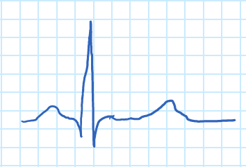
Figura 1. Onda de ECG.

A onda “P” corresponde à contração atrial, e o complexo “QRS” à contração dos ventrículos. O complexo “QRS” é muito maior do que a onda “P” devido à relativa dfferência na massa muscular dos atria e ventrículos, o que mascara o relaxamento do atria. O relaxamento dos ventrículos pode ser visto na forma da onda “T”.

Existem três principais leads responsáveis por medir a diferença de potencial elétrico entre braços e pernas, como mostra a Figura 2. Nesta demonstração, um dos fios do membro, chumbo I, será examinado, e a diferença potencial elétrica entre dois braços será registrada. Como em todas as medidas de chumbo ECG, o eletrodo conectado à perna direita é considerado o nó do solo. Um sinal ECG será adquirido usando um amplificador biopotencial e, em seguida, exibido usando software de instrumentação, onde um controle de ganho será criado para ajustar sua amplitude. Finalmente, o ECG registrado será analisado.

Figure 2
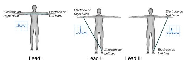
Figura 2. O membro do ECG leva.

Principles

O eletrocardiograma deve ser capaz de detectar não apenas sinais extremamente fracos que variam de 0,5 mV a 5,0 mV, mas também um componente DC de até ±300 mV (resultante do contato eletrodo-pele) e um componente de modo comum de até 1,5 V, o que resulta do potencial entre os eletrodos e o solo. A largura de banda útil de um sinal ECG depende do aplicativo e pode variar de 0,5-100 Hz, às vezes chegando a até 1 kHz. É geralmente em torno de 1 mV de pico ao pico na presença de ruído externo de alta frequência muito maior, interferência de 50 ou 60 Hz, e potencial de deslocamento de eletrodo DC. Outras fontes de ruído incluem movimento que afeta a interface pele-eletrodo, contrações musculares ou picos eletromiográficos, respiração (que pode ser rítmica ou esporádica), interferência eletromagnética (EMI) e ruído de outros dispositivos eletrônicos que acoplam à entrada.

Primeiro, um amplificador biopotencial será produzido para processar o ECG. Em seguida, eletrodos serão colocados no paciente para medir a diferença potencial entre dois braços. A principal função de um amplificador biopotencial é pegar um sinal elétrico fraco de origem biológica e aumentar sua amplitude para que possa ser processado, gravado ou exibido.

Figure 3
Figura 3. Amplificador ECG.

Para serem úteis biologicamente, todos os amplificadores biopotenciais devem atender a certos requisitos básicos:

  • Eles devem ter alta impedância de entrada para que forneçam o carregamento mínimo do sinal sendo medido. Eletrodos biopotenciais podem ser afetados por sua carga, o que leva à distorção do sinal.
  • O circuito de entrada de um amplificador biopotencial também deve fornecer proteção ao sujeito que está sendo estudado. O amplificador deve ter circuitos de isolamento e proteção para que a corrente através do circuito de eletrodos possa ser mantida em níveis seguros.
  • O circuito de saída conduz a carga, que geralmente é um dispositivo de indicação ou gravação. Para obter fidelidade máxima e alcance na leitura, o amplificador deve ter baixa impedância de saída e ser capaz de fornecer a energia necessária pela carga.
  • Os amplificadores biopotenciais devem operar no espectro de frequências no qual os biopotenciais que eles amplificam existem. Devido ao baixo nível desses sinais, é importante limitar a largura de banda do amplificador para obter a relação de sinal ideal para ruído. Isso pode ser feito usando filtros.

A Figura 3 é um exemplo de amplificador ECG, e a Figura 4 é o circuito do amplificador ECG que é construído durante esta demonstração. Possui três estágios principais: o circuito de proteção, o amplificador de instrumentação e o filtro de passagem alta.

Figure 4
Figura 4. Amplificador biopotencial.

O primeiro estágio é o circuito de proteção ao paciente. Um diodo é um dispositivo semicondutor que conduz a corrente em uma direção. Quando um diodo é tendencioso para a frente, o diodo age como um curto-circuito e conduz eletricidade. Quando um diodo é invertido, ele age como um circuito aberto e não conduz eletricidade, eur ≈ 0.

Quando os diodos estão na configuração com viés para a frente, há uma tensão conhecida como tensão limiar (VT = aproximadamente 0,7 V) que deve ser excedida para que o diodo conduza corrente. Uma vez que o VT tenha sido excedido, a queda de tensão através do diodo permanecerá constante em VT, independentemente do que Vestá.

Quando o diodo for com viés reverso, o diodo agirá como em circuito aberto e a queda de tensão através do diodo será igual a Vem.

A Figura 5 é um exemplo de um circuito de proteção simples baseado em diodos que serão usados nesta demonstração. O resistor é usado para limitar a corrente que flui através do paciente. Se uma falha no amplificador de instrumentação ou diodos curto-circuitos da conexão do paciente com um dos trilhos de energia, a corrente seria inferior a 0,11 mA. Os diodos fDH333 de baixo vazamento são usados para proteger as entradas do amplificador de instrumentação. Sempre que a tensão no circuito exceder 0,8 V de magnitude, os diodos mudam para sua região ativa ou estado “ON”; a corrente flui através deles e protege tanto o paciente quanto os componentes eletrônicos.

Figure 6
Figura 5. Circuito de proteção.

O segundo estágio é o amplificador de instrumentação, IA, que utiliza três amplificadores operacionais (op-amp). Há um op-amp ligado a cada entrada para aumentar a resistência à entrada. O terceiro op-amp é um amplificador diferencial. Esta configuração tem a capacidade de rejeitar interferências referidas por terra e apenas amplificar a diferença entre os sinais de entrada.

Figure 7
Figura 6. Amplificador de instrumentação.

O terceiro estágio é o filtro de passagem alta, que é usado para amplificar uma pequena tensão CA que anda em cima de uma grande tensão DC. O ECG é afetado por sinais de baixa frequência que vêm do movimento e respiração do paciente. Um filtro de passagem alta reduz esse ruído.

Filtros de passagem alta podem ser realizados com circuitos RC de primeira ordem. A Figura 7 mostra um exemplo de um filtro de alta-passagem de primeira ordem e sua função de transferência. A frequência de corte é dada pela seguinte fórmula:

Equation 1,Equation 2
Equation 3  Figure 8
Figure 9

Figura 7. Filtro de passagem alta.

Procedure

1. Aquisição de um sinal ECG Ajuste a tensão das fontes para +5 V e -5 V e conecte-as em série. Construa o circuito mostrado na Figura 4. Calcule os valores dos resistores e capacitores. Para o filtro de passagem alta, a frequência de corte deve ser de 0,5 Hz. O valor do capacitor deve ser escolhido na tabela abaixo (de acordo com a disponibilidade). Valores do capacitor disponível (μF ) 0.001 1 100 0.022 2.2 220 0.047 4.7 470 0.01 10 1000 0.1 47 2200 Coloque eletrodos no braço direito, braço esquerdo e perna direita (isto é referência) do paciente, e conecte-os ao circuito. Use o osciloscópio para visualizar o sinal ECG (Vo). Pressione autoto e ajuste as escalas horizontais e verticais conforme necessário. Você deve ser capaz de ver os picos R apesar do barulho no sinal. 2. Exibindo o sinal ECG usando o software de instrumentação Nesta demonstração usamos o LabVIEW. Escreva um programa que exibe o sinal ECG usando uma interface gráfica para configurar medições e um gráfico de forma de onda. Uma vez selecionada uma entrada analógica, configure o programa com as seguintes configurações: Faixa de entrada de sinal >> Max = 0,5; Min = -0,5 Configuração do terminal >> RSE Modo de aquisição >> contínuo Amostras para ler = 2000 Taxa amostral = 1000 Adquira o sinal ECG e observe a forma de onda. Você verá um sinal semelhante à Figura 1. Ajuste a escala do eixo x para mostrar o tempo em segundos. Muitas vezes é necessário na instrumentação amplificar o sinal de interesse para uma amplitude específica. Crie um controle de ganho e defina-o para que a amplitude do ECG seja de 2 Vp. 3. Analisando o sinal ECG Nesta seção, um sinal ECG será filtrado e analisado para determinar a frequência cardíaca. O diagrama do bloco a seguir mostra os componentes do programa. Use um gráfico de forma de onda para exibir o sinal. Avalie o espectro do sinal usando o subvi amplitude e espectro de fase (em processamento de sinal → Espectral) e exiba sua magnitude usando um gráfico de forma de onda. O eixo horizontal corresponde à frequência. É discreto porque o computador usa um algoritmo Fast Fourier Transform (FFT) para calcular o espectro do sinal. A frequência vai de k = 0 a k = (N-1)/2, onde N é o comprimento da sequência, neste caso 4000. Para calcular a frequência analógica correspondente, use a seguinte fórmula:onde fs é a frequência de amostragem. Note que a maior parte da energia do sinal está na faixa de baixa frequência e também que há um pico de alta intensidade na faixa de média frequência. Calcule a frequência desse pico usando a fórmula fornecida acima. Implemente um filtro de baixa passagem usando funções butterworth de Chebyshev. Escolha uma frequência de corte igual a 100 Hz. Certifique-se de que o filtro fornece uma atenuação de pelo menos -60 dB/década na banda de parada. Conecte o sinal de saída da leitura do subvi da planilha à entrada do filtro de baixa passagem. Implemente um filtro de banda parada usando funções Butterworth ou Chebyshev. O objetivo é reduzir a interferência de 60 Hz sem modificar as outras frequências. Experimente frequências fronteiriças perto de 60 Hz. Conecte a saída do filtro lowpass à entrada do filtro stopband. Encontre os picos usando o subvi detector de pico (ele está localizado no processamento de sinal → Operação Sig). Para o limiar, olhe para a amplitude do sinal e escolha o valor mais adequado. Extrair os locais dos picos usando o subvi de matriz de índice (em Programming → Array). Subtrair a posição inferior da posição mais alta, então, multiplique pelo período amostral T = 1/fs para obter o intervalo de RR. Calcule as unidades recíprocas e ajuste e coloque um indicador para exibir o BPM.

Results

In this demonstration, three electrodes were connected to an individual, and the output passed through a biopotential amplifier. A sample ECG graph prior to digital filtering is shown below (Figure 8).

Figure 13
Figure 8. ECG signal without digital filtering.

After designing the filters and feeding the data to the developed algorithm, the peaks on the graph were detected and used to calculate heart beat rate (BPM). Figure 9 displays the raw data an ECG signal (before any filtering) in time and frequency domain. Figure 10 shows the result of filtering that signal.

Figure 11

Figure 9. ECG signal before filtering.

Figure 14
Figure 10. Filtered ECG signal.

The original ECG plot had slightly visible P, QRS, and T complexes that presented many fluctuations from the noise. The spectrum of the ECG signal also showed a clear spike at 65 Hz, which was assumed to be noise. When the signal was processed using a low-pass filter to remove extraneous high frequency portions and then a band-stop filter to remove the 65 Hz signal component, the output appeared significantly cleaner. The ECG shows each component of the signal clearly with all noise removed.

In addition, the measured heart rate was approximately 61.8609 beats per minute.

Applications and Summary

Contraction of cardiac muscle during the heart cycle produces electric currents within the thorax. Voltage drops across resistive tissue are detected by electrodes placed on the skin and recorded by an electrocardiograph. Since the voltage is weak, in the range of 0.5 mV, and small compared to the magnitude of noise, processing and filtering the signal is necessary. In this experiment, an electrocardiograph device consisting of a two part analog and digital signal processing circuit was designed to analyzing the resulting ECG signal, and calculate the heartbeat rate.

This demonstration introduced the fundamentals of electronic circuitry and filtering of ECG signals. Here, practical signal processing techniques were used to extract a weak signal from a noisy background. These techniques can be used in other similar applications where signal amplification and noise reduction is required.

Materials List

Name Company Catalog Number Comments
Equipment
Power supply B&K Precision 1760A
Multimeter
Oscilloscope
Proto-board
4 FDH333 diodes
1 AD620
3 47k resistor
2 100nF capacitors
3 ECG electrodes
Several alligator clips and Tektronix probe.

成績單

Electrocardiographs record cardiac activity of the heart and are used to diagnose disease, detect abnormalities, and learn about overall heart function. Electrical signals are produced by contractions in the heart walls which drive electrical currents and create different potentials throughout the body. By placing electrodes on the skin, one can detect and record this electrical activity in an ECG. ECGs are non-invasive, making them a useful tool to assess how well a patients heart is performing, such as by measuring how well blood flows to the organ.

This video will illustrate the principals of ECGs and demonstrate how to acquire, process, and analyze a typical ECG signal using a biopotential amplifier. Other biomedical applications that utilize electrical signal processing to diagnose disease will also be discussed.

To understand the principles of an ECG, let’s first understand how the heart produces electrical signals. For a normal, healthy heart, at rest, an ECG displays a series of waves that reflect the different phases of a heartbeat. The ECG starts in the sinoatrial node, also known as the SA node, which is located in the right atrium and acts as a pacemaker in the heart. The electrical signals cause atrial contraction forcing blood into the ventricles. This sequence is recorded as the P wave on the ECG. This signal then passes from the atria across the ventricles, causing them to contract and pump blood to the rest of the body. This is recorded as the QRS complex.

Finally, the ventricles relax and this is recorded as the T wave. The process then begins again and is repeated for every heartbeat. Notice that the QRS wave is much larger than the P wave, this is because the ventricles are larger than the atria. Meaning they mask the relaxation of the atria or the T wave. Other processes in the body, like respiration or muscle contractions, can interfere with the ECG measurement. As can currents from the circuitry used to obtain them. Often, the electrical signals that the ECG is attempting to record are quite weak. Therefor, a biopotential amplifier is used to increase their amplitude which allows them to be further processed and recorded.

There are three main components to the biopotential amplifier, the patient protection stage, the instrumentation amplifier, and the high pass filter. As the main suggests, the patient protection circuit uses a combination of resistors and diodes to protect, both, the patient and the machine and equipment. The resistors limit the current that flows through the patient, where as the diodes keep the current flowing in the correct direction.

The next stage is the instrumentation amplifier, which amplifies the difference between the inputs from each electrode. It is composed of three operational amplifiers. Two to increase the resistance from each input, and the third to amplify the difference between the input signals.

The last stage is the high pass filter, which reduces the noise and filters out low frequency signals arising from patient movement or respiration. Now that you know how an ECG is measured, let’s see how to construct a biopotential amplifier and process the data to get a clean ECG signal.

Having reviewed the main principals of electrocardiography, let’s see how to build a biopotential amplifier and acquire an ECG signal. To begin, first gather a proto-board, an AD-620 instrumentation amplifier, and all necessary circuit components. Then, calculate the values of all of the resistors and capacitors in the circuit using the following equation.

For the high pass filter, the cut off frequency should be 0.5 hertz.

Then, plug in the capacitor value to determine the resistance. Next, build a biopotential amplifier according to the provided diagram. Here is what the final circuit should look like. Attach three wires with alligator clips to the binding posts of a DC power supply, then turn on the power source. Adjust the voltage to plus five volts and minus five volts, and connect the the wires, in series, to the circuit.

Now, use an alcohol prep pad to wipe the patients right wrist, left wrist, and right ankle. Add conductive adhesive gel to the electrodes before placing them on the patient. Then, connect the electrodes to the circuit using wires with alligator clips. Turn on the oscilloscope and acquire the ECG signal. Adjust the horizontal and vertical scales as needed. With these adjustments, you should be able to see the R peak of the wave form.

Connect the circuit to the PXI chassis, then open the instrumentation software and, either, use or write a program that will display the ECG signal and a wave form graph.

Configure the data acquisition interface with the following settings. Label the scale of the x-axis to display time and seconds, then display the ECG signal as a waveform. If the signal needs to be amplified, create a gain control and set it so that the amplitude of the ECG is two VP.

Now that we have demonstrated how to acquire an ECG signal, let’s see how to analyze the results. Here is a representative ECG signal. The P, QRS, and T waves are barely discernible because they are obscured by noise and fluctuations. This signal needs to be filtered. To transform this signal, first, select Signal Processing then Spectral on the menu. A Fast Fourier Transform algorithm calculates and plots the spectrum of the signal displaying the frequency as discreet values on the horizontal axis. Most of the energy in the signal is at low frequencies.

But, there is a high intensity peak in the medium frequency range, which is assumed to be noise. Frequency is plotted as k on the horizontal axis and goes from zero to N minus one over two, where N is the length of the sequence. For this experiment, N equals 2,000. Calculate the analog frequency for each k value using the following equation, where f s is the sampling frequency and determine the frequency of the high intensity peak based on the FFT graph.

Then, create a low pass filter with a cutoff frequency of 100 hertz. Use, either, the Butterworth or Chebyshev function to filter the signal, which should attenuate at least 60 decibels per decade in the stop band. Connect the output signal of the data sub VI to the input of the low pass filter. This filter removes the extraneous high frequency waves of the ECG. Now, create a Bandstop filter and set the cutoff frequencies at around 55 and 70 hertz.

To remove the noisy signal, around 60 hertz. Then, connect the output of the low pass filter to the input of the Bandstop filter. Try border frequencies that are close to 60 hertz. This will reduce interference without effecting other frequencies. The ECG signal should now be clear with distinct P, QRS, and T complexes.

Now, let’s determine the heart rate using the filtered ECG signal. First, use the peak detector sub VI to find the peaks of the signal. Choose the most appropriate value based on the signals amplitude of the R wave for the threshold. Then, use the Index Array sub VI to determine the location of the peaks.

Subtract the lower peak position from the higher position, then multiply this value by the sampling period, T, which is equal to one over f s. This value is the length of time between two R waves. Adjust the units to determine the beats per minute.

In this demonstration, the measured heart rate was approximately 60 beats per minute.

ECG and signal processing have important applications in, both, medicine and research. In addition to being non-invasive, ECGs are relatively inexpensive. Making it a useful and accessible tool in hospitals. ECGs can even be adapted to more complex and longterm monitoring of patients who are being treated for Acute Coronary Syndrome.

For this, 12 ECG leads are used, which can identify transient myocardial ischemia in asymptomatic patients. Signal sampling and processing is also used in electroencephalography to measure electrical signals from the brain. EEGs are commonly used in conjunction with functional MRI as a multimodal imaging technique.

The method noninvasively generates cortical maps of brain activity for many neuroimaging applications, such as after visual or motor activation.

You’ve just watched Jove’s introduction to acquiring and analyzing ECG signals. You should now understand how an ECG signal is produced and how to create a biopotential amplifier to detect weak electrical signals. You have also seen some biomedical applications of signal processing for medical diagnosis.

Thanks for watching.

Tags

Cite This
JoVE Science Education Database. JoVE Science Education. Acquisition and Analysis of an ECG (electrocardiography) Signal. JoVE, Cambridge, MA, (2023).