JoVE 科学教育
Biomedical Engineering
This content is Free Access.
JoVE 科学教育 Biomedical Engineering
Acquisition and Analysis of an ECG (electrocardiography) Signal
  • 00:07概述
  • 01:12Principles of Electrocardiography
  • 04:07Building a Biopotential Amplifier and Acquiring an ECG Signal
  • 06:26Filtering an ECG Signal
  • 08:48Results
  • 09:40Applications
  • 10:45Summary

רכישה וניתוח של אות אק"ג (אלקטרוקרדיוגרפיה)

English

分享

概述

מקור: פיימן שהביגי-רודפושטי וסינה שהבזמהאמדי, המחלקה להנדסה ביו-רפואית, אוניברסיטת קונטיקט, סטוררס, קונטיקט

אלקטרוקרדיוגרפיה היא גרף המתועד על ידי שינויים פוטנציאליים חשמליים המתרחשים בין אלקטרודות שהונחו על פלג פלג עליון של המטופל כדי להדגים פעילות לבבית. אות אק”ג עוקב אחר קצב הלב ומחלות לב רבות, כגון זרימת דם לקויה ללב וחריגות מבניות. פוטנציאל הפעולה שנוצר על ידי התכווצויות של דופן הלב פורש זרמים חשמליים מהלב בכל הגוף. הזרמים החשמליים המתפשטים יוצרים פוטנציאלים שונים בנקודות בגוף, אשר ניתן לחוש על ידי אלקטרודות המונחות על העור. האלקטרודות הן מתמרים ביולוגיים העשויים ממתכות ומלחים. בפועל, 10 אלקטרודות מחוברות לנקודות שונות על הגוף. קיים הליך סטנדרטי לרכישה וניתוח אותות אק”ג. גל אק”ג טיפוסי של אדם בריא הוא כדלקמן:
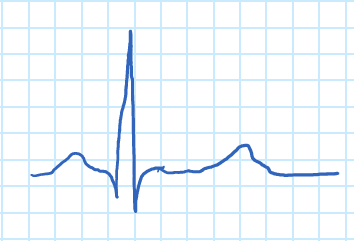
Figure 1
איור 1. גל אק”ג.

גל ה-P מתאים להתכווצות האיזורים, ולמתחם ה-QRS להתכווצות החדרים. מתחם ה-QRS גדול בהרבה מגל ה-P בשל ההצטמרות היחסית במסת השריר של האטריה והחדרים, המסווה את ההרפיה של האטריה. הרפיה של החדרים ניתן לראות בצורה של גל “T”.

ישנם שלושה כיווני חקירה עיקריים האחראים למדידת ההבדל הפוטנציאלי החשמלי בין הידיים לרגליים, כפי שמוצג באיור 2. בהדגמה זו, אחד ממובילי הגפיים, עופרת I, ייבדק, וההבדל הפוטנציאלי החשמלי בין שתי זרועות יירשם. כמו בכל מדידות עופרת אק”ג, האלקטרודה המחוברת לרגל ימין נחשבת לצומת הקרקע. אות אק”ג יירכש באמצעות מגבר ביופוטנציאלי ולאחר מכן יוצג באמצעות תוכנת מכשור, שם תיווצר בקרת רווח כדי להתאים את המשרעת שלה. לבסוף, האק”ג המוקלט ינותח.

Figure 2
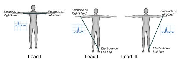
איור 2. עופרת גפיים א.ק.ג.

Principles

האלקטרוקרדיוגרפיה חייבת להיות מסוגלת לזהות לא רק אותות חלשים מאוד הנעים בין 0.5 mV ל 5.0 mV, אלא גם רכיב DC של עד ±300 mV (הנובע ממגע האלקטרודה-עור) ורכיב במצב משותף של עד 1.5 V, הנובע מהפוטנציאל בין האלקטרודות לקרקע. רוחב הפס השימושי של אות אק”ג תלוי ביישום ויכול לנוע בין 0.5-100 הרץ, לפעמים להגיע עד 1 kHz. זה בדרך כלל סביב 1 mV שיא לשיא בנוכחות רעש הרבה יותר גדול בתדר גבוה חיצוני, הפרעות 50 או 60 הרץ, ופוטנציאל היסט אלקטרודה DC. מקורות רעש אחרים כוללים תנועה המשפיעה על ממשק האלקטרודה-עור, התכווצויות שרירים או קוצים אלקטרומיוגרפיים, נשימה (שעשויה להיות קצבית או לא סדירה), הפרעה אלקטרומגנטית (EMI) ורעש ממכשירים אלקטרוניים אחרים המצמידים לקלט.

ראשית, מגבר ביופוטנציאלי יופק לעיבוד האק”ג. לאחר מכן, אלקטרודות יונחו על המטופל כדי למדוד את ההבדל הפוטנציאלי בין שתי זרועות. הפונקציה העיקרית של מגבר ביופוטנציאלי היא לקחת אות חשמלי חלש ממוצא ביולוגי ולהגדיל את המשרעת שלו, כך שניתן יהיה לעבד אותו עוד יותר, להקליט או להציג אותו.

Figure 3
איור 3. מגבר אק”ג.

כדי להיות שימושי מבחינה ביולוגית, כל המגברים הביופוטנטיים חייבים לעמוד בדרישות בסיסיות מסוימות:

  • הם חייבים להיות בעליעכבת קלט גבוהה, כך שהם מספקים טעינה מינימלית של האות הנמדד. אלקטרודות ביופוטנציאליות יכולות להיות מושפעות מהעומס שלהן, מה שמוביל לעיוות האות.
  • מעגל הכניסה של מגבר ביופוטנציאלי חייב גם לספק הגנה לנושא הנחקר. המגבר צריך להיות מעגלי בידוד והגנה, כך הזרם דרך מעגל האלקטרודה ניתן לשמור ברמות בטוחות.
  • מעגל הפלט מניע את העומס, שהוא בדרך כלל התקן מציין או הקלטה. כדי להשיג נאמנות מרבית וטווח בקריאה, המגבר חייב להיות בעל עכבה פלט נמוכה ולהיות מסוגל לספק את הכוח הנדרש על ידי העומס.
  • מגברים ביופוטנטיים חייבים לפעול בספקטרום התדרים שבו קיימים הביופוטנציאלים שהם מגבירים. בגלל הרמה הנמוכה של אותות כאלה, חשוב להגביל את רוחב הפס של המגבר כדי לקבל יחס אות לרעש אופטימלי. ניתן לעשות זאת באמצעות מסננים.

איור 3 הוא דוגמה למגבר א.ק.ג. איור 4 הוא המעגל של מגבר האק”ג שנבנה במהלך הדגמה זו. יש לו שלושה שלבים עיקריים: מעגל ההגנה, מגבר המכשור ומסנן המעבר הגבוה.

Figure 4
איור 4. מגבר ביופוטנציאלי.

השלב הראשון הוא מעגלי ההגנה על המטופלים. דיודה היא התקן מוליכים למחצה המוליך זרם בכיוון אחד. כאשר הדיודה מוטה קדימה, הדיודה פועלת כקצר חשמלי ומוליך חשמל. כאשר דיודה מוטה לאחור, היא פועלת כמעגל פתוח ואינה מוליכת חשמל,אני ≈ 0.

כאשר דיודות נמצאות בתצורה מוטה קדימה יש מתח המכונה מתח הסף (VT = כ 0.7 V) כי יש לחרוג על מנת הדיודה לנהל זרם. לאחר VT כבר חריגה, ירידת המתח על פני הדיודה יישאר קבוע בVT ללא קשר מה Vהוא.

כאשר הדיודה מוטה לאחור הדיודה תפעל כמו במעגל פתוח וירידת המתח על פני הדיודה תהיה שווה ל- Vב.

איור 5 הוא דוגמה למעגל הגנה פשוט המבוסס על דיודות שישמשו בהדגמה זו. הנגד משמש להגבלת הזרם הזורם דרך המטופל. אם תקלה במגבר המכשור או בדיודות מקצרת את החיבור של המטופל לאחת מפסי החשמל, הזרם יהיה פחות מ-0.11 מיליאמפר-אם-איי. דיודות הדליפה הנמוכה FDH333 משמשות להגנה על התשומות של מגבר המכשור. בכל פעם שהמתח במעגל עולה על 0.8 V בסדר גודל, הדיודות משתנות לאזור הפעיל שלהן או למצב “ON”; הזרם זורם דרכם ומגן הן על המטופל והן על הרכיבים האלקטרוניים.

Figure 6
איור 5. מעגל הגנה.

השלב השני הוא מגבר המכשור, IA, המשתמש בשלושה אמפרים תפעוליים (op-amp). יש מגבר אופ אחד המחובר לכל קלט כדי להגביר את התנגדות הקלט. המגבר השלישי הוא מגבר דיפרנציאלי. לתצורה זו יש את היכולת לדחות הפרעות המופנות לקרקע ורק להגביר את ההבדל בין אותות הקלט.

Figure 7
איור 6. מגבר מכשור.

השלב השלישי הוא מסנן המעבר הגבוה, המשמש להגברת מתח AC קטן שרוכב על גבי מתח DC גדול. האק”ג מושפע מאותות בתדר נמוך המגיעים מתנועת המטופלים ומנשימה. מסנן מעבר גבוה מפחית רעש זה.

מסנני מעבר גבוהים יכולים להתממש עם מעגלי RC מסדר ראשון. איור 7 מציג דוגמה למסנן מעבר גבוה מסדר ראשון ולפונקציית ההעברה שלו. תדירות הניתוק ניתנת על-ידי הנוסחה הבאה:

Equation 1,Equation 2
Equation 3  Figure 8
Figure 9

איור 7. מסנן מעבר גבוה.

Procedure

1. רכישת אות אק”ג התאם את המתח של המקורות ל+ 5 V ו- -5 V וחבר אותם בסדרה. בנו את המעגל המוצג באיור 4. חשב את הערכים של הנגדים והחיברים. עבור מסנן המעבר הגבוה, תדירות הניתוק צריכה להיות 0.5 הרץ. יש לבחור את ערך הקבל מהטבלה שלהלן (בכפוף לזמינות). ערכי קבלים זמינים (μF ) 0.001 1 100 0.022 2.2 שנות ה-12 0.047 4.7 470 0.01 10 1000 0.1 47 2200 מניחים אלקטרודות על זרוע ימין, זרוע שמאל ורגל ימין (זוהי התייחסות) של המטופל, וחברו אותם למעגל. השתמש באוסצילוסקופ כדי להציג את אות האק”ג (Vo). הקש על הגדר אוטומטית והתאם את קנה המידה האופקי והאנכי לפי הצורך. אתה אמור להיות מסוגל לראות את פסגות R למרות הרעש באות. 2. הצגת אות האק”ג באמצעות תוכנת מכשור בהדגמה זו השתמשנו ב- LabVIEW. כתוב תוכנית המציגה את אות האק”ג באמצעות ממשק גרפי לתצורת מדידות וגרף צורת גל. לאחר בחירת קלט אנלוגי, קבע את תצורת התוכנית עם ההגדרות הבאות: טווח קלט אותות >> מקסימום = 0.5; מינימום = -0.5 >> תצורת מסוף RSE מצב רכישה >> רציף דוגמאות לקריאה = 2000 קצב דגימה = 1000 לרכוש את אות האק”ג ולהתבונן צורת הגל. תראה אות דומה לאיור 1. כוונן את קנה המידה של ציר ה- x כדי להציג זמן בשניות. לעתים קרובות יש צורך מכשור כדי להגביר את האות של עניין משרעת ספציפית. צור בקרת רווח והגדר אותה כך שהמשרעת של האק”ג היא 2 סמנכ”לים. 3. ניתוח אות האק”ג בסעיף זה, אות אק”ג יעבור סינון וניתוח כדי לקבוע את קצב הלב. דיאגרמת החסימה הבאה מציגה את רכיבי התוכנית. השתמש בגרף צורת גל כדי להציג את האות. להעריך את הספקטרום של האות באמצעות משרעת ואת ספקטרום הפאזה subvi (בעיבוד אותות → ספקטרלי) ולהציג את גודלו באמצעות גרף צורת גל. הציר האופקי תואם לתדר. הוא דיסקרטי מכיוון שהמחשב משתמש באלגוריתם של שינוי פורייה מהיר (FFT) כדי לחשב את הספקטרום של האות. התדירות עוברת מ- k = 0 ל- k = (N-1)/2, כאשר N הוא אורך הרצף, במקרה זה 4000. כדי לחשב את התדירות האנלוגית המתאימה, השתמש בנוסחה הבאה:כאשר fs הוא תדר הדגימה. שים לב שרוב האנרגיה של האות היא בטווח התדרים הנמוכים וגם שיש שיא של עוצמה גבוהה בטווח התדרים הבינוני. חשב את התדירות של פסגה זו באמצעות הנוסחה שסופקה לעיל. ליישם מסנן נמוך לעבור באמצעות באטרוורת ‘ של פונקציות Chebyshev. בחר תדירות חיתוך השווה ל- 100 הרץ. ודא שהמסנן מספק נכה של לפחות -60 dB/עשור בפס העצירה. חבר את אות הפלט של הקריאה מ- subvi גיליון אלקטרוני לקלט של מסנן המעבר הנמוך. יש ליישם מסנן סטופ-פס באמצעות פונקציות באטרוורת’ או צ’בישב. המטרה היא להפחית את ההפרעה של 60 הרץ מבלי לשנות את התדרים האחרים. נסה תדרי גבול קרוב ל- 60 הרץ. חבר את הפלט של מסנן lowpass לקלט של מסנן פס העצירה. מצא את הפסגות באמצעות subvi גלאי שיא (הוא ממוקם עיבוד אותות → פעולת סיג). עבור הסף, הסתכלו על משרעת האות ובחרו את הערך המתאים ביותר. חלץ את מיקומי הפסגות באמצעות subvi מערך האינדקס (במערך → תכנות). הפחת את המיקום התחתון ממיקום גבוה יותר ולאחר מכן, הכפל בתקופת הדגימה T = 1/fs כדי להשיג את מרווח הזמן של RR. חשב את יחידות ההדדיות והתאם וצב מחוון כדי להציג את ה- BPM.

Results

In this demonstration, three electrodes were connected to an individual, and the output passed through a biopotential amplifier. A sample ECG graph prior to digital filtering is shown below (Figure 8).

Figure 13
Figure 8. ECG signal without digital filtering.

After designing the filters and feeding the data to the developed algorithm, the peaks on the graph were detected and used to calculate heart beat rate (BPM). Figure 9 displays the raw data an ECG signal (before any filtering) in time and frequency domain. Figure 10 shows the result of filtering that signal.

Figure 11

Figure 9. ECG signal before filtering.

Figure 14
Figure 10. Filtered ECG signal.

The original ECG plot had slightly visible P, QRS, and T complexes that presented many fluctuations from the noise. The spectrum of the ECG signal also showed a clear spike at 65 Hz, which was assumed to be noise. When the signal was processed using a low-pass filter to remove extraneous high frequency portions and then a band-stop filter to remove the 65 Hz signal component, the output appeared significantly cleaner. The ECG shows each component of the signal clearly with all noise removed.

In addition, the measured heart rate was approximately 61.8609 beats per minute.

Applications and Summary

Contraction of cardiac muscle during the heart cycle produces electric currents within the thorax. Voltage drops across resistive tissue are detected by electrodes placed on the skin and recorded by an electrocardiograph. Since the voltage is weak, in the range of 0.5 mV, and small compared to the magnitude of noise, processing and filtering the signal is necessary. In this experiment, an electrocardiograph device consisting of a two part analog and digital signal processing circuit was designed to analyzing the resulting ECG signal, and calculate the heartbeat rate.

This demonstration introduced the fundamentals of electronic circuitry and filtering of ECG signals. Here, practical signal processing techniques were used to extract a weak signal from a noisy background. These techniques can be used in other similar applications where signal amplification and noise reduction is required.

Materials List

Name Company Catalog Number Comments
Equipment
Power supply B&K Precision 1760A
Multimeter
Oscilloscope
Proto-board
4 FDH333 diodes
1 AD620
3 47k resistor
2 100nF capacitors
3 ECG electrodes
Several alligator clips and Tektronix probe.

成績單

Electrocardiographs record cardiac activity of the heart and are used to diagnose disease, detect abnormalities, and learn about overall heart function. Electrical signals are produced by contractions in the heart walls which drive electrical currents and create different potentials throughout the body. By placing electrodes on the skin, one can detect and record this electrical activity in an ECG. ECGs are non-invasive, making them a useful tool to assess how well a patients heart is performing, such as by measuring how well blood flows to the organ.

This video will illustrate the principals of ECGs and demonstrate how to acquire, process, and analyze a typical ECG signal using a biopotential amplifier. Other biomedical applications that utilize electrical signal processing to diagnose disease will also be discussed.

To understand the principles of an ECG, let’s first understand how the heart produces electrical signals. For a normal, healthy heart, at rest, an ECG displays a series of waves that reflect the different phases of a heartbeat. The ECG starts in the sinoatrial node, also known as the SA node, which is located in the right atrium and acts as a pacemaker in the heart. The electrical signals cause atrial contraction forcing blood into the ventricles. This sequence is recorded as the P wave on the ECG. This signal then passes from the atria across the ventricles, causing them to contract and pump blood to the rest of the body. This is recorded as the QRS complex.

Finally, the ventricles relax and this is recorded as the T wave. The process then begins again and is repeated for every heartbeat. Notice that the QRS wave is much larger than the P wave, this is because the ventricles are larger than the atria. Meaning they mask the relaxation of the atria or the T wave. Other processes in the body, like respiration or muscle contractions, can interfere with the ECG measurement. As can currents from the circuitry used to obtain them. Often, the electrical signals that the ECG is attempting to record are quite weak. Therefor, a biopotential amplifier is used to increase their amplitude which allows them to be further processed and recorded.

There are three main components to the biopotential amplifier, the patient protection stage, the instrumentation amplifier, and the high pass filter. As the main suggests, the patient protection circuit uses a combination of resistors and diodes to protect, both, the patient and the machine and equipment. The resistors limit the current that flows through the patient, where as the diodes keep the current flowing in the correct direction.

The next stage is the instrumentation amplifier, which amplifies the difference between the inputs from each electrode. It is composed of three operational amplifiers. Two to increase the resistance from each input, and the third to amplify the difference between the input signals.

The last stage is the high pass filter, which reduces the noise and filters out low frequency signals arising from patient movement or respiration. Now that you know how an ECG is measured, let’s see how to construct a biopotential amplifier and process the data to get a clean ECG signal.

Having reviewed the main principals of electrocardiography, let’s see how to build a biopotential amplifier and acquire an ECG signal. To begin, first gather a proto-board, an AD-620 instrumentation amplifier, and all necessary circuit components. Then, calculate the values of all of the resistors and capacitors in the circuit using the following equation.

For the high pass filter, the cut off frequency should be 0.5 hertz.

Then, plug in the capacitor value to determine the resistance. Next, build a biopotential amplifier according to the provided diagram. Here is what the final circuit should look like. Attach three wires with alligator clips to the binding posts of a DC power supply, then turn on the power source. Adjust the voltage to plus five volts and minus five volts, and connect the the wires, in series, to the circuit.

Now, use an alcohol prep pad to wipe the patients right wrist, left wrist, and right ankle. Add conductive adhesive gel to the electrodes before placing them on the patient. Then, connect the electrodes to the circuit using wires with alligator clips. Turn on the oscilloscope and acquire the ECG signal. Adjust the horizontal and vertical scales as needed. With these adjustments, you should be able to see the R peak of the wave form.

Connect the circuit to the PXI chassis, then open the instrumentation software and, either, use or write a program that will display the ECG signal and a wave form graph.

Configure the data acquisition interface with the following settings. Label the scale of the x-axis to display time and seconds, then display the ECG signal as a waveform. If the signal needs to be amplified, create a gain control and set it so that the amplitude of the ECG is two VP.

Now that we have demonstrated how to acquire an ECG signal, let’s see how to analyze the results. Here is a representative ECG signal. The P, QRS, and T waves are barely discernible because they are obscured by noise and fluctuations. This signal needs to be filtered. To transform this signal, first, select Signal Processing then Spectral on the menu. A Fast Fourier Transform algorithm calculates and plots the spectrum of the signal displaying the frequency as discreet values on the horizontal axis. Most of the energy in the signal is at low frequencies.

But, there is a high intensity peak in the medium frequency range, which is assumed to be noise. Frequency is plotted as k on the horizontal axis and goes from zero to N minus one over two, where N is the length of the sequence. For this experiment, N equals 2,000. Calculate the analog frequency for each k value using the following equation, where f s is the sampling frequency and determine the frequency of the high intensity peak based on the FFT graph.

Then, create a low pass filter with a cutoff frequency of 100 hertz. Use, either, the Butterworth or Chebyshev function to filter the signal, which should attenuate at least 60 decibels per decade in the stop band. Connect the output signal of the data sub VI to the input of the low pass filter. This filter removes the extraneous high frequency waves of the ECG. Now, create a Bandstop filter and set the cutoff frequencies at around 55 and 70 hertz.

To remove the noisy signal, around 60 hertz. Then, connect the output of the low pass filter to the input of the Bandstop filter. Try border frequencies that are close to 60 hertz. This will reduce interference without effecting other frequencies. The ECG signal should now be clear with distinct P, QRS, and T complexes.

Now, let’s determine the heart rate using the filtered ECG signal. First, use the peak detector sub VI to find the peaks of the signal. Choose the most appropriate value based on the signals amplitude of the R wave for the threshold. Then, use the Index Array sub VI to determine the location of the peaks.

Subtract the lower peak position from the higher position, then multiply this value by the sampling period, T, which is equal to one over f s. This value is the length of time between two R waves. Adjust the units to determine the beats per minute.

In this demonstration, the measured heart rate was approximately 60 beats per minute.

ECG and signal processing have important applications in, both, medicine and research. In addition to being non-invasive, ECGs are relatively inexpensive. Making it a useful and accessible tool in hospitals. ECGs can even be adapted to more complex and longterm monitoring of patients who are being treated for Acute Coronary Syndrome.

For this, 12 ECG leads are used, which can identify transient myocardial ischemia in asymptomatic patients. Signal sampling and processing is also used in electroencephalography to measure electrical signals from the brain. EEGs are commonly used in conjunction with functional MRI as a multimodal imaging technique.

The method noninvasively generates cortical maps of brain activity for many neuroimaging applications, such as after visual or motor activation.

You’ve just watched Jove’s introduction to acquiring and analyzing ECG signals. You should now understand how an ECG signal is produced and how to create a biopotential amplifier to detect weak electrical signals. You have also seen some biomedical applications of signal processing for medical diagnosis.

Thanks for watching.

Tags

Cite This
JoVE Science Education Database. JoVE Science Education. Acquisition and Analysis of an ECG (electrocardiography) Signal. JoVE, Cambridge, MA, (2023).